Math in Focus

This handy Math in Focus Grade 8 Workbook Answer Key Chapter 10 Lesson 10.3 Two-Way Tables detailed solutions for the textbook questions.

Math in Focus Grade 8 Course 3 B Chapter 10 Lesson 10.3 Answer Key Two-Way Tables

Math in Focus Grade 8 Chapter 10 Lesson 10.3 Guided Practice Answer Key

Solve.

Question 1.
A survey asked 1,000 gym members what type of exercises they do when they visit the gym. The results are recorded in a two-way table as shown.

a) Find the total number of male gym members surveyed.
Total number of males = Total surveyed – Total number of females
= –
=
The total number of male gym members surveyed is .
Answer:
Total number of males = Total surveyed – Total number of females
= 1000 – 481
= 519
The total number of male gym members surveyed is 519.

b) Find the number of male gym members who chose both types of exercises.
Number of males who chose both
= Total number of males – Number of males who chose cardios – Number of males who chose weights
= – –
=
The number of male gym members who chose both types of exercises is .
Answer:
Number of males who chose both
= Total number of males – Number of males who chose cardios – Number of males who chose weights
= 519 – 125 – 279
= 115
The number of male gym members who chose both types of exercises is 115.

c) Find the total number of gym members who chose cardio exercises.
Total number of members who chose cardios
= Number of males who chose cardios + Number of female who chose cardios
= ___ +____
= __
The total number of gym members who chose cardio exercises is ___.
Answer:
Total number of members who chose cardios
= Number of males who chose cardios + Number of female who chose cardios
= 125 +295
= 420
The total number of gym members who chose cardio exercises is 420.

Question 2.
An athletic club owner wants to know which cardio exercise is most popular: cycling, running, or swimming. The owner is also interested in whether athletic club members read sports magazines. He surveys 20 randomly selected athletic club members. Results are shown below.

C represents cycling
R represents running
S represents swimming
Y represents read sports magazines
N represents do not read sports magazines

a) Summarize the data into a two-way table.
Answer:

b) Which cardio exercise do club members prefer?
The total number of members who chose cycling, running, and swimming is , , and respectively. So members prefer .
Answer:
By seeing the above table we can know how many members prefer cardio exercise.
The total number of members who chose cycling, running, and swimming is 6, 9, and 5 respectively. So members prefer running.

c) What percent of club members read sports magazines?
The total number of club members surveyed is .
The number of people that read sports magazines is .
Percent of participants that read sports magazines is .
Answer:
The total number of club members surveyed is 20.
The number of people that read sports magazines is 10.
Percent of participants that read sports magazines is 50%.

d) Describe any association between the type of cardio exercise that the club members prefer and whether the members read sports magazines.
The number of cyclists, runners, and swimmers that read sports magazines is , , and . So, more prefer to read sports magazines.
There is association between the type of cardio exercise that the club members prefer and whether the members read sports magazines.
Answer:
The number of cyclists, runners, and swimmers that read sports magazines is 5, 2, and 3. So, more cyclists prefer to read sports magazines.
There is no association between the type of cardio exercise that the club members prefer and whether the members read sports magazines.

Copy the table. Solve. Round your answer to the nearest hundredth where necessary.

Question 3.
A survey asked 1,000 gym members what type of exercises they do when they visit the gym. The results are recorded into a two-way table as shown.

a) Find the relative frequencies to compare the distribution of genders among each type of exercises.

Answer:

b) Describe the distribution of male and female gym members for each type of exercises.
More members do cardio exercises than members.
More members do weight exercises than members. Among those who do both types of exercises, it is distributed between male and female gym members, with slightly more  members.
Answer:
More female members do cardio exercises than male members.
More male members do weight exercises than female members. Among those who do both types of exercises, it is almost evenly distributed between male and female gym members, with slightly more female members.

c) Find the relative frequencies to compare the distribution of the type of exercises among each gender.

Answer:

d) Describe the distribution of male and of female gym members for each type of exercises.
Among male members, most do exercises and least do exercises.
Among female members, most do exercises and least do exercises.
Answer:
Among male members, most do weight exercises and least do both exercises.
Among female members, most do cardio exercises and least do weight exercises.

Math in Focus Course 3B Practice 10.3 Answer Key

Identify the categorical data.

Question 1.
Temperature, Weight, Color
Answer: Color

Question 2.
Street name, Number of boxes. Time
Answer: Street name

Identify whether the given data is categorical or quantitative.

Question 3.
Large, medium, small
Answer: categorical

Question 4.
20 mi/h, 40 mi/h, 50 mi/h
Answer: quantitative

Use the two-way table to answer questions 5 to 9.

In some states, all passengers in a vehicle are required to wear a seat belt when the vehicle is on a public road. A poll of 275 randomly selected vehicle passengers was conducted in a state that has the seat belt law to determine the association between passengers who know the seat belt law and passengers who obey this law.

Question 5.
Find the number of passengers who wear seat belts.
Answer:
Number of passengers = Total randomly selected vehicle passengers – Number of passengers not wearing seat belts.
275 – 50 = 225

Question 6.
Find the number of passengers who wear seat belts and do not know the seat belt law.
Answer:

Question 7.
Find the number of passengers who do not wear seat belts and know the seat belt law.
Answer: 50 – 15 = 35

Question 8.
Describe what you can see in the data from the row totals and column totals.
Answer: From the table, we observe the number of passengers who wear seat belts and the number of passengers who know seat belt law.

Question 9.
Is there any association between the passengers who know the seat belt law and passengers who obey the seat belt law?
Answer: From the table, we observe the number of passengers who know the seat belt law and passengers who obey the seat belt law.

Use the data below to answer questions 10 to 12.

A survey of 24 households shows whether they save a portion of their income regularly and whether they have life insurance.

S represents save regularly
NS represents do not save regularly
L represents have life insurance
NL represents do not have life insurance

Question 10.
Arrange the above data into a two-way table.
Answer:
The objective of this task is to make a two-way table of the survey about whether the household has a life insurance and if they regularly save a part of their salary.

Since there are two categories in the survey, whether they save regularly a portion of their earnings and if they have life insurance, then the two-way table will be divided into this categories. Observe that there are 8 homes that has savings and insurance, 3 homes do not have savings but they have life insurance and another 3 have savings but do not have life insurance. Lastly, there are 10 households that do not have both savings and life insurance.

Question 11.
Do more or fewer households have life insurance than not? Support your answer with the given data.
Answer:
The target of this task is to compare the number of household that has a life insurance and to does who does not have.

Observe the two-way table. Notice that there are 11 houses that have life insurance and 13 who does not have. Therefore, there are fewer households that acquire life insurance than do not have.

Question 12.
Is there any association between households that save regularly and households that have life insurances? Justify your answer from the data.
Answer:
The goal is to verify the relation of the households that regularly save a portion of their income to the homes with life insurance.

Households with savings tend to have life insurance compared to households who do not save since there are 8 households who have savings and insurance, but only 3 households who do not have savings and possess a life insurance.

Use the table to answer questions 13 to 15.

The table below shows whether the sales target of salesperson are met and whether they are paid on commission.

Question 13.
Find the relative frequencies among the rows, and interpret their,L meanings. Round your answer to the nearest hundredth where necessary.
Answer:
245/330 = 0.74
85/330 = 0.26
12/76 = 0.16
64/76 = 0.84

Question 14.
Find the relative frequencies among the columns, and interpret their meanings. Round your answer to the nearest hundredth where necessary.
Answer:
245/257 = 0.95
12/257 = 0.04
85/149 = 0.57
64/149 = 0.43

Question 15.
Describe the association between a salesperson meeting the sales target and whether the salesperson is paid on commission.
Answer:
Salesperson those who are not paid on commission tend not to meet the sales target, while salesperson who are paid on commission tend to meet the sales target.

Brain @Work

Question 1.
Mindy was shown two scatter plots.
a) The diagram below shows the first scatter plot.

Mindy concluded that there is a linear association between the bivariate data. But her teacher told her she is wrong. Explain why her teacher says so.
Answer: We can see some data missing points in the above graph between the interval that has no data points, it may not be necessary to follow linear trend.

b) The diagram below shows the second scatter plot.

Mindy concluded that there is a linear association between the bivariate data. Her teacher disagree with her. Explain why.
Answer:
There are only 3 data points and that is an insufficient amount of data to conclude the association between the bivariate data.

Question 2.
A school principal conducted research to find out about students learning a second language and students learning music. He surveyed 500 students, and the relative frequencies of the data are shown below.

a) The total number of students who are learning second language is 200. Find the total number of students who are and who are not learning music.
Answer: 200 × 90/100 = 180
200 × 10/100 = 20
500 – 200 = 300
300 × 45/100 = 135
300 × 55/100 = 165
total number of students who are not learning music = 20 + 165 = 185
total number of students who are learning music = 180 + 135 = 315

b) Represent the actual data in a two-way table.
Answer:

This handy Math in Focus Grade 8 Workbook Answer Key Chapter 10 Lesson 10.2 Modeling Linear Associations detailed solutions for the textbook questions.

Math in Focus Grade 8 Course 3 B Chapter 10 Lesson 10.2 Answer Key Modeling Linear Associations

Hands-On Activity

Materials:
measuring tape

CONSTRUCT AND INTERPRET SCATTER PLOTS

Work in groups of 5.

Background
A person’s height is closely associated with their arm span. In a medical context, this association can be used to estimate realistic lengths for prosthetic limbs. In this activity, you will collect data on the heights and arm spans of classmates.

STEP 1: Measure the arm span of one group member while he or she is standing straight up against a wall with arms stretched out from the body and with all the fingers extended fully. Measure the arm span from the tip of the middle finger of one hand all the way to the other middle finger on the other hand.

STEP 2: While in the same position, use a ruler to mark the member’s height on the wall. While holding the ruler, ask the member to step away so you can measure the height.

STEP 3: Repeat STEP 1 and STEP 2 with the other group members.

STEP 4: Organize the data in a table like the one shown below.

STEP 5: Collect data from all the groups. Construct a scatter plot with the collected data.

Math Journal From the scatter plot drawn, describe any association you see between the height and arms span.
Using the collected data, obtain a measure for the arm span of a schoolmate. Use the scatter plot to predict his or her height. Compare your estimations with the actual measurements to find how accurate the estimate is.
Answer:

Math in Focus Grade 8 Chapter 10 Lesson 10.2 Guided Practice Answer Key

Use graph paper. Solve.

Question 1.
A city collected data over the course of a week to find the association between the number of waste bins per acre, x, in their parks and the pounds of litter collected, y pounds, in each bin. The data is shown below.

a) Construct a scatter plot for this data. Use 1 centimeter on the horizontal axis to represent 2 waste bins per acre for x interval from 8 to 26. Use 1 centimeter on the vertical axis to represent 5 pounds of litter per week. Sketch a line of best fit for the given table of data.
Answer:
Observe that

• 12 bins per acre corresponds to 70 lbs of litter,
• 24 waste bins has 18 pounds of trash,
• 16 waste bins per acre means 50 Lbs. of garbage,
• 10 bins per acre, 66 pounds of litter are coLlected,
• 18 bins per acre corresponds to 42 lbs. of Litter,
• 20 waste bins has 32 pounds of trash,
• 26 waste bins per acre means 12 lbs. of garbage,
• 16 bins per acre, 44 pounds of litter are collected,
• 22 bins per acre corresponds to 26 lbs. of Litter,
• 16 waste bins has 58 pounds of trash,
• 14 waste bins per acre means 62 Lbs. of garbage,
• 22 bins per acre, 30 pounds of litter are collected,
• 10 bins per acre corresponds to 74 lbs. of litter,
• 20 waste bins has 40 pounds of trash,
• 12 waste bins per acre means 62 Lbs. of garbage, and
• 18 bins per acre, 4 pounds of Utter are coLLected.

Note that the Line of best fit is a straight line that best shows the data on a scatter plot Therefore, the scatter plot would be as depicted below.

b) Identify the association and describe the meaning of the association in context.
There is a , , and association between the number of waste bins per acre and the pounds of litter collected per bin.
Answer:
The scatter plot shows a strong, negative and linear association which indicates that the more waste bins per acre in the city the lesser the pounds of litter collected.

c) Identify the outlier and describe the outlier in context.
The data point (, ) is an outlier representing only pounds of litter collected per bin when there are waste bins per acre in the park.
Answer:
The outlier is the data that is very different from the rest in a set Notice the outlier is the point that is away from then line, in this case, observe the best-fit line, then the point isolated to it is at (18, 4). The outlier represents 18 waste bins per acre and a litter of 4 pounds.

Question 2.
A city collected data to find the association between the daily high temperature, x °F, and the number of pool visitors, y, that day. The data is shown below.

Construct a scatter plot for this data. Use 1 centimeter on the horizontal axis to represent 2°F on the x interval from 84 to 98. Use 1 centimeter on the vertical axis to represent 10 pool visitors on the y interval from 220 to 360. Sketch a line that appears to best fit the data and write its equation.
Answer:
The objective is to make a scatter plot daily high temperature and daily pool visitor, give the line of best fit for the scatter plot and the equation for it

Observe that when the temperature is 96 F the pool visitors are 312. a 92° F temperature in the city makes 304 visitors, the city has 256 pool visitors when the temperature is at 86°F, when the temperature is 90° the pool visitors are 284, a 98°F temperature in the city makes 332 visitors, the city has 88 pool visitors when the temperature is at 272°F, when the temperature is 94°F the pool visitors are 320. a 96°F temperature in the city makes 336 visitors, the city has 276 pool visitors when The temperature is at 90°F, when the temperature is 98°F the pool visitors are 340, a 86 F temperature in the city makes 248 visitors, the city has 296 pool visitors when The temperature is at 92°F, when the temperature is 98°F the pool visitors are 360, a 92°F temperature in the city makes 324 visitors, the city has 300 pool visitors when The temperature is at 94°F, and when the temperature is 9W F the pool visitors are 316. Also, note that the line of best fit is the most possibLe straight line that best shows The data on a scatter plot Thus, the scatter plot will be as depicted below.

For the equation of the Line of best fit, first, use points that the best fit line passes through, (86, 248) and (92, 296), to solve for the slope of the line. The slope of the line equates the difference of y₂ to y₁ over the difference of x₂ to x₁. Then, Let in be the slope, (86, 248) be (x₁, y₁) and (92, 296) be (x₂, y₂) so
m = \(\frac{y_{2}-y_{1}}{x_{2}-x_{1}}\)      Slope Formula.
= \(\frac{296-248}{92-86}\)  Substitution.
= \(\frac{48}{6}\)    Subtract.
= 8     Simplify.
Next, use the slope-intercept form to determine the equation of the straight line given by y = mx + b, where in is the slope, b is the y-intercept, and (86, 248) be (x, y) then
y = mx + b     Slope-intercept Form.
248 = 8(86) + b     Substitution.
248 = 688 + b      Multiply.
248 – 688 = 688 + b – 688    Subtract both sides by 688
-440 = b Simplify.
Lastly, using the slope-intercept form again, let m be the sLope equals to 8 and b equals to -440, thus
y = mx + b   Slope-intercept Form.
y = 8x – 440     Substitution.
Therefore, the equation of the line of best fit is y = 8x – 440.

Question 3.
The scatter plot below shows the number of eggs hatched, y, per 100 eggs in an incubator with varying temperatures, x°F.

a) Given that the line of best fit passes through (80, 41) and (95, 68), find the equation of the line of best fit.
First find the slope of the line of best fit that passes through the points (80, 41) and (95, 68).
m = \(\frac{?-?}{?-?}\) = \(\frac{?}{?}\) =
Next find the y-intercept using the equation in slope-intercept form

Finally, write an equation,
y = mx + b
y = x + Substitute for m and for b.
The equation of the line of best fit is .
Answer:
a. To find the equation of the Line, compute for the slope of the Line then substitute it in the slope-intercept form together with one of the points that the line of best fit passes through. From here, b wilL be solved then use the slope-intercept form again substituting only the slope m and y-intercept b.
Determining the slope of the line, let (80. 41) be x₁ and y₁ while (95, 68) be x₂ and y₂. Then,
m = \(\frac{y_{2}-y_{1}}{x_{2}-x_{1}}\)      Formula.
= \(\frac{68-41}{95-80}\)  Substitution.
= \(\frac{27}{15}\)    Subtract.
= 1.8     Simplify.
Now, let (80, 41) be (x, y), and since the slope is equal to 1.8, then,
y = mx + b    Formula.
41 = 1.8(80) + b    Substitution.
41 = 144 + b    Multiply.
41 – 144 = 144 – 144 + b    Subtract 144 From Both Sides.
103 = b    Evaluate.
Since m is equal to 1.8 and b is equal to -103, then
y = mx + b   Slope-Intercept Form.
y = 1.8x + (-103)    Substitution.
y = 1.8x – 103    Simplify.
Therefore, the equation of the line is y = 1.8x – 103.

b) Use the graph to estimate the number of eggs that would hatch per 100 eggs if the temperature of the incubator is kept at 86°F.
About eggs could be predicated to hatch if the incubator is kept at a temperature of .
Answer:
To estimate the number of hatched eggs x and the temperature of the incubator y, study the graph then note at what point does y at 86°F meets x. The point is on (52, 86). Therefore, there are 52 eggs wilt be hatched at 81°F

c) Use the equation to estimate the number of eggs that would hatch per 100 eggs if the temperature of the incubator is kept at 65°F.
Using the equation , substitute for x.
y = • – =
About eggs could be expeced to hatch when the temperature of the incubator is kept at 65°F.
Answer:
To compute the number of eggs hatched at 65°F, note that the equation of the line is y = 1.8x + b, the number of hatched eggs is denoted as y, and temperature of The incubator denoted as x. So let x be 65°F.
y = 1.8x – 103    Formula.
y = 1.8(65) – 103    Substitution.
y = 117 – 103    Multiply.
y = 14     Subtract.
Therefore, there will be 14 hatched eggs at 65°F.

Technology Activity

Materials:
graphing calculator

USE A GRAPHING CALCULATOR TO GRAPH A LINE OF BEST FIT FOR A SCATTER PLOT

Background
In the Hands-On Activity on page 186, you drew a scatter plot for the data on the heights and arm spans of all the groups. In this activity, you will learn how to construct a scatter plot and graph the line of best fit using a graphing calculator.

STEP 1: Press and select 1 : Edit to choose the edit function. Input the data for arm spans in column L1 and the data for heights in column L2. You should have at least 20 data points to interpret the data accurately.

STEP 2: Press , and select 1 to go to the scatter plot setting screen. Under Type, select the scatter plot options as shown.

STEP 3: Press to see the scatter plot.

STEP 4: Press and select CALC, 4: LinReg(ax+b). Press select Y-VARS, 1 : Function and 1 :Y1. Press This step is to find the values of m and b for the line of best fit. In the graphing calculator, the value of m is denoted by a.

STEP 5: Press to see the scatter plot and the line of best fit. Press and select 9: ZoomStat to zoom in the graph.

Math Journal Compare the hand drawn scatter plot and the one drawn using graphing calculator. Is there any difference between the line of best fit drawn by hand and by the graphing calculator? Compare both sets of m and b values. Discuss how you can plot a better line of best fit based on the m and b values obtained using the graphing calculator.
Answer:

Math in Focus Course 3B Practice 10.2 Answer Key

State the line that represents the line of best fit for each scatter plot.

Question 1.

Answer:
The goal of this task is to determine the Line of best fit for the scatter plot.

Line B best fits the scatter plot It is the more possible straight line that best shows the data on a scatter plot compared to Line .4.

Question 2.

Answer:
The objective of this task is to determine the tine of best fit for the scatter plot.

Line C best fits the given scatter plot It is the most possible straight line that best shows the data on a scatter plot in comparison to line 4 and line B.

Construct each scatter plot and draw a line of best fit for each table of bivariate data.

Question 3.
Use 1 centimeter on the horizontal axis to represent 1 unit. Use 1 centimeter on the vertical axis to represent 20 units.

Answer:
The target of this task ¡s to make a scatter plot from the given values of r and y and the tine of best fit for the scatter plot.

Notice that when x is 4 y is 72, if x is equal to 1 y is equal to 12, when is equal to 2 y is 32, if z is 3 y is equal to 164, the value of y is 88 when z is 5. when z is 6 y is 112, if z is equal to 3 y is equal to 52, when z is equal to 6 y is 88, if z is 2 y is equal to 40, and the vaLue of y is 136 when z is 7. Also, the line of best fit is the most a possible straight line that best shows the data on a scatter plot Thus, the scatter plot will be as depicted below.

Question 4.
Use 1 centimeter on the horizontal axis to represent 1 unit for the x interval from 80 to 87. Use 1 centimeter on the vertical axis to represent 10 units for the y interval from 200 to 300.

Answer:
The goal is to make a scatter plot from the given values of z and y and the line of best fit for the scatter plot.

Notice that when z is 80 y is 220, if z is equal to 84 y is equal to 236, when z is equal to 81 y is 214, if z is 87 y is equal to 256, the value of y is 200 when z is 81, when z is 86 y is 250, if z is equal to 82 y is equal to 292, when z is equal to 83 y is 220, if z is 83 y is equal to 240, the value of y is 238 when z is 84. when z is 85 y is 240, x is equal to 85 y is equal to 244, when z is equal to 83 y is 232 and if z is equal to 82 y is equal to 222. Also, the line of best fit is the most possible straight line that best shows the data on a scatter plot Thus, the scatter plot wilt be as depicted below.

Question 5.
Use 1 centimeter on the horizontal axis to represent 0.1 unit. Use 1 centimeter on the vertical axis to represent 5 units for the y interval from 20 to 70.

Answer:
The objective is to make a scatter plot from the given values of x and y and the line of best fît for the scatter plot

Notice that when r is 0.1 y is 69, if x is equal to 0.9 y is equal to 59, when x is equal to 0.3 y is 66, if x is 0.4 y is equal to 65, the value of y is 64 when x is 0.4, when x is 1.1 y is 58, if z is equal to 1.0 y is equal to 61, when x is equal.to 0.8 y is 59, if x is 0.5 y is equal to 65, the value of y is 63 when x is 0.7, when x is 0.7 y is 60, if x is equal to 0.6 y is equal to 30, when x is equal to 0.2 y is 68 and if x is equal to 0.5 y is equal to 62. Also, the line of best fit is the most possible straight line that best shows the data on a scatter plot Thus, the scatter plot will be as depicted below.

Construct a scatter plot and draw a line of best fit for each table of bivariate data. Find an equation of the line of best fit.

Question 6.
Use 2 centimeters on the horizontal axis to represent 1 tree for the x interval from 13 to 18. Use 1 centimeter on the vertical axis to represent 20 squirrels for the y interval from 260 to 480.

Answer:
The task is to make a scatter plot and give the tine of best fit for the number of trees and the population of squirrels then determine the equation of the line.

For the scatter plot determine at which point does the number of trees x meets its corresponding population of the squirrel y according to the table. For the tine of best fit, note that it is the most possible straight line that best shows the data on a scatter plot Thus, the scatter plot will be as depicted below.

For the equation of the line of best fit, use points that the best fit Une passes through, (15. 392) and (16, 420). to solve for the slope of the line. The slope of the line equates the difference of y₂ to y₁ over the difference of x₂ to x₁. Then, let m be the slope, (15, 392) be (x₁, y₁) and (16, 420) be (x₂, y₂) so
m = \(\frac{y_{2}-y_{1}}{x_{2}-x_{1}}\)       Formula.
= \(\frac{420-392}{16-15}\)    Substitution.
= \(\frac{28}{1}\)      Subtract.
= 28    Simplify.
Next use the slope-intercept form to determine the equation of the straight line given by y = mx + b, where ni is the slope, b is the y-intercept, and (15, 392) be (x, y) then
y = mx + b     Slope-intercept Form.
392 = 28(15) + b    Substitution.
392 = 420 + b    Multiply.
392 – 420 = 420 + b – 420     Subtract both sides by 420
-28 = b      Simplify.
Lastly, using the slope-intercept form again, let rn be the slope equals to 28 and b equals to -28. thus
y = mx + b      Slope-intercept Form.
y = 28x – 28    Substitution.
Therefore, the equation of the Une of best fit is y = 28x – 28.

Question 7.
Use 1 centimeter on the horizontal axis to represent 5 kilometers. Use 1 centimeter on the vertical axis to represent 1 liter for the y interval from 5 to 16.

Answer:
The task is to make a scatter plot and give the line of best fit for the distance traveLled and the gasoline used then to determine the equation of the line.

For the scatter plot, determine at which point does the distance x meets the corresponding gasoline used y according to the table. For the tine of best fit, note that it is the most possible straight line that best shows the data on a scatter plot Thus, the scatter plot will be as depicted below.

For the equation of the line of best fit, use points that the best fit line passes through, (37, 8) and (56, 10.2), to solve for the slope of the Line. The slope of the line equates the difference of y₂ to y₁ over the difference of x₂ to x₁. Then, let m be the sLope, (37, 8) be (x₁, y₁) and (56, 10.2) be (x₂. y₂) so
m = \(\frac{y_{2}-y_{1}}{x_{2}-x_{1}}\)       Formula.
= \(\frac{10.2-8}{56-37}\)    Substitution.
= \(\frac{2.2}{19}\)      Subtract.
Next, use the slope-intercept form to determine the equation of the straight line given by y = mx + b, where m is the sLope, b is the y-intercept, and (37, 8) be (x, y) then
y = mx + b      Slope-intercept Form.
8 = (\(\frac{2.2}{19}\))37 + b    Substitution.
8 = (\(\frac{407}{95}\)) + b    Multiply.
(\(\frac{353}{95}\)) = b     Subtract (\(\frac{407}{95}\)) to both sides.
Lastly, using the slope-intercept form again, let m be the slope equals to (\(\frac{2.2}{19}\)) and b equals to (\(\frac{353}{95}\)), thus
y = mx + b    Slope-intercept Form.
y = \(\frac{2.2 x}{19}\) – \(\frac{353}{95}\)      Substitution.
Therefore, the equation of the tine of best fit is y = \(\frac{2.2 x}{19}\) – \(\frac{353}{95}\).

Use the scatter plot below to answer questions 8 to 13.

Snow density is an important factor affecting the speed and control in snow boarding. To understand the relationship between snow density, y grams per cubic centimeters, and air temperature, x°C, data are collected and shown below.

Question 8.
Use graph paper to construct the scatter plot. Use 1 centimeter on the horizontal axis to represent 1°C for the x interval from -17 to -9. Use 1 centimeter on the vertical axis to represent 0.010 grams per cubic centimeter.
Answer:
The objective is to make a scatter plot for the snow density and air temperature.

Observe that when the air temperature is at -17°C the snow density is 0.036g/cm³, at -16° the density is 0.060g/cm³, the air temperature is at -15°C the snow density is 0.050g/cm3, at -14° the density is 0.60g/cm³, the air temperature is at -13°C the snow density is 0.054g/cm³, at -12° the density is 0.070g/cm³. the air temperature is at -11°C the snow density is 0.086g/cm³, and at -10° the density is 0.090g/cm³. Thus, the scatter plot will be as depicted below.

Question 9.
Describe the association between air temperature and snow density.
Answer:
The target is to determine the association in bivariate data then explain the relationship between the two.

The scatter plot shows a weak, positive and linear association. This relationship indicates that the greater the temperature, the higher the snow density.

Question 10.
Sketch a line of best fit.
Answer:
The goal of this task is to determine the line of best fit in the scatter plot of the snow density and air temperature.

Observe that when the air temperature is at -17°C the snow density is 0.036g/cm³, at 16 the density is 0.060g/cm³. the air temperature is at -15°C the snow density is 0.050g/cm³, at -14° the density is 0.060g/cm³, the air temperature is at -13°C the snow density is 0.054g/cm³, at -12° the density is 0.070g/cm³. the air temperature is at -11°C the snow density is 0.086g/cm³, and at -10° the density is 0.090g/cm³. Also, the line of best fit is the most possible straight line that best shows the data on a scatter plot Thus, the line of best fit for scatter plot will be as depicted below.

Question 11.
Find an equation for the line of best fit.
Answer:
The objective of this task is to determine the equation of the Line of best fit for the air temperature and snow density.

Notice that the best fit Une passes through (-14, 0.060) and (- 12.0.070). Use these points to solve for the slope of the line which equates the difference of y₂ to y₁ over the difference of x₂ to x₁. Then, let m be the slope, (-14,0.060) be (x₁, y₁) and (-12,0.070) be (x₂. y₂) so
m = \(\frac{y_{2}-y_{1}}{x_{2}-x_{1}}\)    Slope Formula.
= \(\frac{0.070-0.060}{(-12)-(-14)}\)    Substitution.
= \(\frac{0.01}{2}\) Subtract.
= 0.005 Simplify.
Next use the slope-intercept form to determine the equation of the straight line given by y = mx + b, where w is the slope, b is the y-intercept, and (-14,0.060) be (x, y) then
y = mx + b    Slope-intercept Form.
0.060 = (0.005)(-14) + b    Substitution.
0.060 = -0.07 + b   Multiply.
0.060 + 0.07 = -0.07 + b + 0.07    Add 0.07 to both sides.
b = 0.13 Simplify.
Lastly, using the slope-intercept form again, let w be the slope equals to 0.005 and b equals to 0.13. thus
y = mx + b     Slope-intercept Form.
y = 0.005x + 0.13   Substitution
Therefore, the equation of the line of best fit is y = 0.005x + 0.13.

Question 12.
Predict the density when the temperature is at -14.5°C.
Answer:
The target of this task is to give the approximate snow density using the graph if the temperature is at -14.6°C.

To estimate the snow density x given the air temperature y, study the graph and the tine of best fit then note at what point does y at -14°C meets x. The point is on (-14.6, 0.062).

Therefore, at an air temperature of -14°C, the snow density is around 0.062g/cm³.

Question 13.
Predict the density when the temperature is at -9°C.
Answer:
The goal is to calculate using the equation of the Line y = 0.005x + 0.13 the snow density if the air temperature is at -9°C.

To compute the snow density at -9°C, note that snow density is denoted as y and the air temperature is denoted as x. Then when x is -9,
y = 0.005x + 0.13    Equation of the line.
= 0.005(-9) + 0.13     Substitution.
= -0.045 + 0.13    Multiply.
= 0.085   Simplify.

Therefore, when using the equation y = 0.005x + 0.13 the snow density is about 0.085 at a temperature of -9°C.

This handy Math in Focus Grade 8 Workbook Answer Key Chapter 10 Lesson 10.1 Scatter Plots detailed solutions for the textbook questions.

Math in Focus Grade 8 Course 3 B Chapter 10 Lesson 10.1 Answer Key Scatter Plots

Math in Focus Grade 8 Chapter 10 Lesson 10.1 Guided Practice Answer Key

Use graph paper. Solve.

Question 1.
The table shows some monetary exchanges between U.S. dollars, x dollars, and Japanese yen, y yen, over a time period of 4 months at a major airport.

Construct a scatter plot for this data. Use 2 centimeters on the horizontal axis to represent $10. Use 2 centimeters on the vertical axis to represent 500 yen.
Answer:

Complete.

Question 2.
Describe the association between the bivariate data shown in each scatter plot.

Graph E: and association
Graph F: , , and association
Graph G: association
Answer:
Graph E: strong and non-linear association
Graph F: Strong, Positive, and linear association
Graph G: No association

Use graph paper. Solve.

Question 3.
Dan is investigating the effect of the amount of water, x, given to tomato seedlings on their growth. He waters each of the 22 plants with a given amount of water daily. He records their height, y, at the end of two weeks. His data is shown below.

a) Construct a scatter plot for this data. Use 1 centimeter on the horizontal axis to represent 4 fluid ounce. Use 1 centimeter on the vertical axis to represent 1 inch. Identify any outlier(s).
An outlier appears to be located at (, ).
Answer:

An outlier appears to be located at (28, 4.8).

b) Explain what the outlier(s) likely represent(s) in this context.
The outlier represents and after two weeks.
Answer: The outlier represents 28 fluid ounces of water daily and a growth of 4.8 inches after two weeks.

c) Describe the meaning in context of the association between the two data sets. Validate the outliers as being very different from the rest of the data points.
The , , and association indicates that tomato seedlings that are given more water daily experience growth over the two weeks. The general trend shows that seedlings that are given 28 fluid ounces of water daily generally grew about inches, but the outlier represents a seedling that grew only inches with fluid ounces of water daily.
Answer:
The strong, positive, and linear association indicates that tomato seedlings that are given more water daily experience more growth over the two weeks. The general trend shows that seedlings that are given 28 fluid ounces of water daily generally grew about 12 inches to 13 inches, but the outlier represents a seedling that grew only 4.8 inches with 28 fluid ounces of water daily.

Math in Focus Course 3B Practice 10.1 Answer Key

Draw scatter plot for each of the given table of bivariate data.

Question 1.
Use 1 centimeter on the horizontal axis to represent 10 units. Use 1 centimeter on the vertical axis to represent 20 units.

Answer:

Question 2.
Use 1 centimeter on the horizontal axis to represent 5,000 people. Use 2 centimeters on the vertical axis to represent 5,000 cars.

Answer:

Question 3.
Use 1 centimeter on the horizontal axis to represent 1 hour. Use 1 centimeter on the vertical axis to represent a score of 10.

Answer:

Describe the association between the bivariate data shown in each scatter plot.

Question 4.

Answer: Strong, linear and positive

Question 5.

Answer: Strong, linear and negative

Describe the association between the bivariate data shown in each scatter plot.

Question 6.

Answer: strong, nonlinear and positive

Question 7.

Answer: Strong, negative and nonlinear

Identify the outlier(s) in each scatter plot.

Question 8.

Answer: (1, 1) and (4, 1)

Question 9.

Answer: (0, 1) and (5, 0.4)

Use the table of bivariate data below to answer questions 10 to 13.

A retailer wanted to know the association between the number of items sold, y, and the number of salespeople, x, in a store. So she recorded the number of salesperson and items sold over 16 days in the table below.

Question 10.
Use graph paper to construct the scatter plot. Use 1 centimeter on the horizontal axis to represent 1 salesperson for the x interval from 43 to 52. Use 1 centimeter on the vertical axis to represent 20 items.
Answer:

Question 11.
Identify the outlier. Give a likely explanation for the occurrence of the outlier.
Answer: (50, 52) because there could have been an accident or construction that blocked the access to the store for a long time that day.

Question 12.
Describe the association between the number of items sold and the number of salespeople in the store. Explain your answer.
Answer: The wide range of sampling values might be important when investigating the association between bivariate data

Question 13.
Math Journal If the data collected for the number of salespeople ranged from 0 to 100, do you think the answer to 12 would be different? Explain why a wide range of sampling values might be important when investigating the association between bivariate data.
Answer: If the association occurs over a greater range of values, then the narrow range if value might not be enough to identify the data.

Use the table of data below to answer questions 14 to 17.

To investigate the benefits of warming up before playing a baseball game, 14 amateur baseball players were surveyed. The number of game injuries, x, in a year and the time the player spent warming up for each game, y minutes, are recorded below.

Question 14.
Use graph paper to construct the scatter plot. Use 2 centimeters on the horizontal axis to represent 1 minute. Use 1 centimeter on the vertical axis to represent 5 game injuries.
Answer:

Question 15.
Identify any outliers.
Answer: no

Question 16.
Math journal Is there a linear association between the number of game injuries and the time spent warming up before each game? Explain.
Answer:
The task is to verify if there exist a linear association in the scatter plot for the number of game injuries and the time spent in warming up. If the scatter plot follows a straight line then it is linear, otherwise, it has a nonlinear association. Observe that there is a liner association in the scatter plot because as the time spent in warming up increases, the number of game injuries increases and thus the marks of these variables have a negative linear association

Question 17.
Math Journal From the results shown, can you recommend minimum : warm-up time for baseball players before they start a game? How does
analyzing association of data sets help to provide useful information?
Answer:
The target of this task is to give a suggestion about how long should the players warm-up, and then make a conclusion about the importance of studying the relationship of a group of data. Observe the scatter plot of the number of minutes players warm-up and the number of injuries. From 1 – 3 minutes, the behavior of data shows that as the time increases, the recorded injuries decreases. When the Length of warming up enters 4 the number of injuries are almost the same even at Longer warming-up time. Therefore, the shortest warming-up time is 4 minutes. A good analyzation of a group of data helps in making a good prediction.

This handy Math in Focus Grade 8 Workbook Answer Key Chapter 10 Statistics detailed solutions for the textbook questions.

Math in Focus Grade 8 Course 3 B Chapter 10 Answer Key Statistics

Math in Focus Grade 8 Chapter 10 Quick Check Answer Key

Solve.

Question 1.
The table shows the numbers of students involved in four sports at a high school. Find the relative frequency for each sport.

Answer:
Relative frequency is the probability of an event occurring based on all possible events.

This handy Math in Focus Grade 7 Workbook Answer Key Chapter 9 Review Test detailed solutions for the textbook questions.

Math in Focus Grade 7 Course 2 B Chapter 9 Review Test Answer Key

Concepts and Skills

Find the range, the three quartiles, and the interquartile range.

Question 1.
2, 4, 1, 7, 3, 3, 9, 10, 1, 0, 6, 8, 5, 5, 9
Answer:
The range in statistics for a given data set is the difference between the highest and lowest values.
Range=maximum observation-minimum observation
how to find range:
To find the range in statistics, we need to arrange the given values or set of data or set of observations in ascending order. That means, firstly write the observations from the lowest to the highest value. Now, we need to use the formula to find the range of observations.
Ascending order:
0, 1, 1, 2, 3, 3, 4, 5, 5, 6, 7, 8, 9, 9, 10
Maximum value=10
Minimum value=0
range=10-0
range=10
Quartiles:
Quartiles mark each 25% of a set of data:
1. The first quartile Q₁ is the 25th percentile
2. The second quartile Q₂ is the 50th percentile
3. The third quartile Q₃ is the 75th percentile
The second quartile Q₂ is easy to find. It is the median of any data set and it divides an ordered data set into upper and lower halves.
Data set: 0, 1, 1, 2, 3, 3, 4, 5, 5, 6, 7, 8, 9, 9, 10
Q2=5
The first quartile Q₁ is the median of the lower half not including the value of Q₂. The third quartile Q₃ is the median of the upper half not including the value of Q₂.
n=15 (odd)
0, 1, 1, 2, 3, 3, 4
If the size of the data set is odd, do not include the median when finding the first and third quartiles.
Q1=2
Q3 data set: 5, 6, 7, 8, 9, 9, 10
Q3=8
Interquartile range=Q3-Q1
Interquartile range=8-2
Interquartile range=6

Question 2.
34, 66, 90, 25, 46, 81, 40, 67, 95, 104, 36, 49
Answer:
The range in statistics for a given data set is the difference between the highest and lowest values.
Range=maximum observation-minimum observation
how to find range:
To find the range in statistics, we need to arrange the given values or set of data or set of observations in ascending order. That means, firstly write the observations from the lowest to the highest value. Now, we need to use the formula to find the range of observations.
Ascending order:
25, 34, 36, 40, 46, 49, 66, 67, 81, 90, 95, 104
Maximum value=104
Minimum value=25
Range=104-25
Range=79
Quartiles:
Quartiles mark each 25% of a set of data:
1. The first quartile Q₁ is the 25th percentile
2. The second quartile Q₂ is the 50th percentile
3. The third quartile Q₃ is the 75th percentile
The second quartile Q₂ is easy to find. It is the median of any data set and it divides an ordered data set into upper and lower halves.
Data set=25, 34, 36, 40, 46, 49, 66, 67, 81, 90, 95, 104
Q2=49+66/2
Q2=115/2
Q2=57.5
The first quartile Q₁ is the median of the lower half not including the value of Q₂. The third quartile Q₃ is the median of the upper half not including the value of Q₂.
Q1 data set: 25, 34, 36, 40, 46, 49
Q1=36+40/2
Q1=76/2
Q1=38
Q1 is the median of the lower half of the data.
Q3 data set: 66, 67, 81, 90, 95, 104
Q3=81+90/2
Q3=171/2
Q3=85.5
Interquartile range=Q3-Q1
Interquartile range=85.5-38
Interquartile range=47.5

Question 3.
1.23, 1.45, 1.09, 1.78, 1.55, 1.67, 1.37, 1.05, 1.23, 1.11
Answer:
The range in statistics for a given data set is the difference between the highest and lowest values.
Range=maximum observation-minimum observation
how to find range:
To find the range in statistics, we need to arrange the given values or set of data or set of observations in ascending order. That means, firstly write the observations from the lowest to the highest value. Now, we need to use the formula to find the range of observations.
Ascending order:
1.05, 1.09, 1.11, 1.23, 1.23, 1.37, 1.45, 1.55, 1.67, 1.78
Maximum value=1.78
Minimum value=1.05
Range=1.78-1.05
Range=0.73
Quartiles:
Quartiles mark each 25% of a set of data:
1. The first quartile Q₁ is the 25th percentile
2. The second quartile Q₂ is the 50th percentile
3. The third quartile Q₃ is the 75th percentile
The second quartile Q₂ is easy to find. It is the median of any data set and it divides an ordered data set into upper and lower halves.
Data set: 1.05, 1.09, 1.11, 1.23, 1.23, 1.37, 1.45, 1.55, 1.67, 1.78
Q2=1.23+1.37/2
Q2=2.6/2
Q2=1.3
The first quartile Q₁ is the median of the lower half not including the value of Q₂. The third quartile Q₃ is the median of the upper half not including the value of Q₂.
Q1 data set: 1.05, 1.09, 1.11, 1.23, 1.23
Q1=1.11
Q3 data set: 1.37, 1.45, 1.55, 1.67, 1.78
Q3=1.55
Interquartile range=Q3-Q1
Interquartile range=1.55-1.11
Interquartile range=0.44

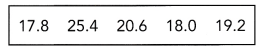
Question 4.
162.5, 248.6, 130.7, 344.9, 322.0, 234.2, 150.8, 304.7, 326.4
Answer:
The range in statistics for a given data set is the difference between the highest and lowest values.
Range=maximum observation-minimum observation
how to find range:
To find the range in statistics, we need to arrange the given values or set of data or set of observations in ascending order. That means, firstly write the observations from the lowest to the highest value. Now, we need to use the formula to find the range of observations.
Ascending order:
130.7, 150.8, 162.5, 234.2, 248.6, 304.7, 322.0, 326.4, 344.9
Maximum value=344.9
Minimum value=130.7
Range=344.9-130.7
Range=214.2
Quartiles:
Quartiles mark each 25% of a set of data:
1. The first quartile Q₁ is the 25th percentile
2. The second quartile Q₂ is the 50th percentile
3. The third quartile Q₃ is the 75th percentile
The second quartile Q₂ is easy to find. It is the median of any data set and it divides an ordered data set into upper and lower halves.
Data set: 130.7, 150.8, 162.5, 234.2, 248.6, 304.7, 322.0, 326.4, 344.9
Q2= 248.6
n=9 (odd)
If the size of the data set is odd, do not include the median when finding the first and third quartiles.
The first quartile Q₁ is the median of the lower half not including the value of Q₂. The third quartile Q₃ is the median of the upper half not including the value of Q₂.
Q1 data set: 130.7, 150.8, 162.5, 234.2
Q1=150.8+162.5/2
Q1=313.3/2
Q1=156.65
Q3 data set: 304.7, 322.0, 326.4, 344.9
Q3=322.0+326.4/2
Q3=648.4/2
Q3=324.2
Interquartile range=Q3-Q1
Interquartile range=324.2-156.65
Interquartile range=167.55

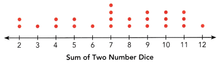
Use the information below to answer the following.

Tara tossed two number dice 24 times. She found the sum of the values for each throw and displayed the sums in a dot plot.

Question 5.
Find the range of the data.
Answer:
The range in statistics for a given data set is the difference between the highest and lowest values.
Range=maximum observation-minimum observation
how to find range:
To find the range in statistics, we need to arrange the given values or set of data or set of observations in ascending order. That means, firstly write the observations from the lowest to the highest value. Now, we need to use the formula to find the range of observations.
According to the dot plot the data set will be:
2, 2, 3, 4, 4, 5, 5, 6, 7, 7, 7, 7, 8, 8, 9, 9, 9, 10, 10, 10, 11, 11, 11, 12.
maximum value=12
minimum value=2
Range=12-2
Range=10

Question 6.
Find the 3 quartiles of the data.
Answer:
Quartiles:
Quartiles mark each 25% of a set of data:
1. The first quartile Q₁ is the 25th percentile
2. The second quartile Q₂ is the 50th percentile
3. The third quartile Q₃ is the 75th percentile
The second quartile Q₂ is easy to find. It is the median of any data set and it divides an ordered data set into upper and lower halves.
The given data set: 2, 2, 3, 4, 4, 5, 5, 6, 7, 7, 7, 7, 8, 8, 9, 9, 9, 10, 10, 10, 11, 11, 11, 12.
Q2=7+8/2
Q2=15/2
Q2=7.5
The first quartile Q₁ is the median of the lower half not including the value of Q₂. The third quartile Q₃ is the median of the upper half not including the value of Q₂.
Q1 data set: 2, 2, 3, 4, 4, 5, 5, 6, 7, 7, 7, 7
Q1=5+5/2
Q1=10/2
Q1=5
Q1 is the median of the lower half of the data.
Q3 data set: 8, 8, 9, 9, 9, 10, 10, 10, 11, 11, 11, 12
Q3=10+10/2
Q3=20/2
Q3=10
Q3 is the median of the upper half of the data.

Question 7.
Find the interquartile range.
Answer:
The interquartile range defines the difference between the third and the first quartile. Quartiles are the partitioned values that divide the whole series into 4 equal parts. So, there are 3 quartiles. First Quartile is denoted by Q₁ known as the lower quartile, the second Quartile is denoted by Q₂ and the third Quartile is denoted by Q₃ known as the upper quartile. Therefore, the interquartile range is equal to the upper quartile minus the lower quartile.
The difference between the upper and lower quartile is known as the interquartile range. The formula for the interquartile range is given below
Interquartile range = Upper Quartile – Lower Quartile = Q_­3 – Q1
where Q₁ is the first quartile and Q₃ is the third quartile of the series.
Q1=5; Q3=10
Interquartile range=Q3-Q1
Interquartile range=10-5
Interquartile range=5

Solve. Show your work.

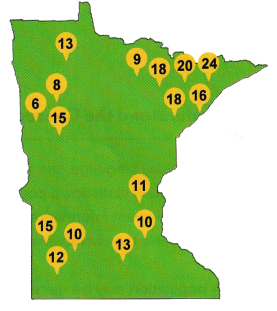
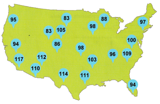
Question 8.
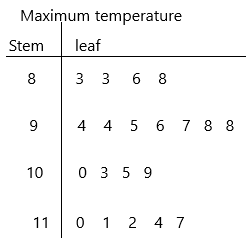
The map shows the maximum temperature, in degrees Fahrenheit, recorded in 20 cities across the United States in a certain year. Display the data in a stem-and-leaf plot.

Answer:

The Stem and Leaf plot is a way of organizing data into a form that makes it easy to see the frequency of different values. In other words, we can say that a Stem and Leaf Plot is a table in which each data value is split into a “stem” and a “leaf.” The “stem” is the left-hand column that has the tens of digits. The “leaves” are listed in the right-hand column, showing all the ones digit for each of the tens, the twenties, thirties, and forties. Remember that Stem and Leaf plots are a pictorial representation of grouped data, but they can also be called a modal representation. Because, by quick visual inspection at the Stem and Leaf plot, we can determine the mode.
Steps for making:
1. First, determine the smallest and largest number in the data.
2. Identify the stems.
3. Draw a with two columns and name them as “Stem” and “Leaf”.
4. Fill in the leaf data.
5. Remember, a Stem and Leaf plot can have multiple sets of leaves.
The given data:95, 94, 117, 110, 112, 86, 83, 105, 83, 114, 111, 103, 98, 98, 88, 96, 109, 100, 97, 94
Ascending order:83, 83, 86, 88, 94, 94, 95, 96, 97, 98, 98, 100, 103, 105, 109, 110, 111, 112, 114, 117

Question 9.
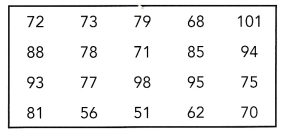
The table shows the weights of Labrador dogs, in pounds.

a) Draw a stem-and-leaf plot for the data.
Answer:
The given data: 72, 73, 79, 68, 101, 88, 78, 71, 85, 94, 93, 77, 98, 95, 75, 81, 56, 51, 62, 70
The Stem and Leaf plot is a way of organizing data into a form that makes it easy to see the frequency of different values. In other words, we can say that a Stem and Leaf Plot is a table in which each data value is split into a “stem” and a “leaf.” The “stem” is the left-hand column that has the tens of digits. The “leaves” are listed in the right-hand column, showing all the ones digit for each of the tens, the twenties, thirties, and forties. Remember that Stem and Leaf plots are a pictorial representation of grouped data, but they can also be called a modal representation. Because, by quick visual inspection at the Stem and Leaf plot, we can determine the mode.
Steps for making:
1. First, determine the smallest and largest number in the data.
2. Identify the stems.
3. Draw a with two columns and name them as “Stem” and “Leaf”.
4. Fill in the leaf data.
5. Remember, a Stem and Leaf plot can have multiple sets of leaves.
Ascending order: 51, 56, 62, 68, 70, 71, 72, 73, 75, 77, 78, 79, 81, 85, 88, 93, 94, 95, 98, 101

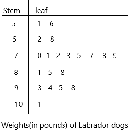
5|1 represents 51 pounds.

b) How many Labrador dogs are there?
Answer:
The given data: 72, 73, 79, 68, 101, 88, 78, 71, 85, 94, 93, 77, 98, 95, 75, 81, 56, 51, 62, 70
the number of given data is equal to number of Labrador dogs.
Now count the numbers present in the sata set.
There are 20 Labrador dogs.

c) What is the range?
Answer:
The range in statistics for a given data set is the difference between the highest and lowest values.
Range=maximum observation-minimum observation
how to find range:
To find the range in statistics, we need to arrange the given values or set of data or set of observations in ascending order. That means, firstly write the observations from the lowest to the highest value. Now, we need to use the formula to find the range of observations.
The given data: 72, 73, 79, 68, 101, 88, 78, 71, 85, 94, 93, 77, 98, 95, 75, 81, 56, 51, 62, 70
Ascending order: 51, 56, 62, 68, 70, 71, 72, 73, 75, 77, 78, 79, 81, 85, 88, 93, 94, 95, 98, 101
Maximum value=101
Minimum value=51
range=101-51
range=50

d) What is the mode of the data?
Answer:
The mode is the observation’s value, which occurs most frequently, i.e., an observation with the maximum frequency is called the mode. A data set can have more than one mode, which means more than one observation has the same maximum frequency.
The given data: 72, 73, 79, 68, 101, 88, 78, 71, 85, 94, 93, 77, 98, 95, 75, 81, 56, 51, 62, 70
Ascending order: 51, 56, 62, 68, 70, 71, 72, 73, 75, 77, 78, 79, 81, 85, 88, 93, 94, 95, 98, 101
Therefore, there is no modal weight. No number doesn’t occur more times.

e) What is the median weight?
Answer:
The median of a set of data is the middlemost number or centre value in the set. The median is also the number that is halfway into the set. To find the median, the data should be arranged, first, in order of least to greatest or greatest to the least value. A median is a number that is separated by the higher half of a data sample, a population or a probability distribution, from the lower half. The median is different for different types of distribution.
Formula:
The formula to calculate the median of the finite number of data set is given here. The median formula is different for even and odd numbers of observations. Therefore, it is necessary to recognise first if we have an odd number of values or an even number of values in a given data set.
The formula to calculate the median of the data set is given as follow.
An odd number of observations:
If the total number of observation given is odd, then the formula to calculate the median is:
Median = {(n+1)/2}^thterm; where n is the number of observations
Even number of observations:
If the total number of observations is even, then the median formula is:
Median  = [(n/2)^th term + {(n/2)+1}^th]/2; where n is the number of observations
The given data: 72, 73, 79, 68, 101, 88, 78, 71, 85, 94, 93, 77, 98, 95, 75, 81, 56, 51, 62, 70
Ascending order: 51, 56, 62, 68, 70, 71, 72, 73, 75, 77, 78, 79, 81, 85, 88, 93, 94, 95, 98, 101
Median=77+78/2
Median=155/2
Median=77.5 lb

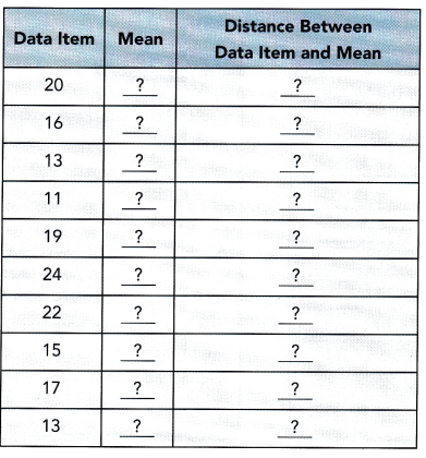
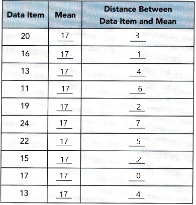
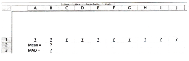
Find the mean absolute deviation.

Question 10.
57, 60, 31, 30, 26, 46, 52, 40, 35, 60
Answer:
To understand Mean Absolute Deviation, let us split both the words and try to figure out their meaning. ‘Mean’ refers to the average of the observations and deviation implies departure or variation from a preset standard. When put together, we can define mean deviation as the mean distance of each observation from the mean of the data.
formula:
The ratio of the sum of all absolute values of deviation from central measure to the total number of observations.
M.A. D = (Σ Absolute Values of Deviation from Central Measure) / (Total Number of Observations)
Calculate MAD:
Steps to find the mean deviation from mean:
(i)Find the mean of the given observations.
(ii)Calculate the difference between each observation and the calculated mean
(iii)Evaluate the mean of the differences obtained in the second step.
This gives you the mean deviation from the mean.
The given data set: 57, 60, 31, 30, 26, 46, 52, 40, 35, 60
First, we have to calculate the mean:
Mean= sum of observations/total number of observations
Mean=57+60+31+30+26+46+52+40+35+60/10
Mean=437/10
mean=43.7
Now calculate the difference between each observation and the calculated mean
|57-43.7|=13.3
|60-43.7|=16.3
|31-43.7|=12.7
|30-43.7|=13.7
|26-43.7|=17.7
|46-43.7|=2.3
|52-43.7|=8.3
|40-43.7|=3.7
|35-43.7|=8.7
|60-43.7|=16.3
Now calculate the mean for obtained differences
MAD=13.3+16.3+12.7+13.7+17.7+2.3+8.3+3.7+8.7+16.3/10
MAD=113/13
MAD=11.3

Question 11.
1.46, 2.03, 3.12, 2.55, 4.25, 1.80, 4.08, 2.87
Answer:
To understand Mean Absolute Deviation, let us split both the words and try to figure out their meaning. ‘Mean’ refers to the average of the observations and deviation implies departure or variation from a preset standard. When put together, we can define mean deviation as the mean distance of each observation from the mean of the data.
formula:
The ratio of the sum of all absolute values of deviation from central measure to the total number of observations.
M.A. D = (Σ Absolute Values of Deviation from Central Measure) / (Total Number of Observations)
Calculate MAD:
Steps to find the mean deviation from mean:
(i)Find the mean of the given observations.
(ii)Calculate the difference between each observation and the calculated mean
(iii)Evaluate the mean of the differences obtained in the second step.
This gives you the mean deviation from the mean.
The given data set: 1.46, 2.03, 3.12, 2.55, 4.25, 1.80, 4.08, 2.87
First, we have to calculate the mean:
Mean= sum of observations/total number of observations
Mean=1.46+2.03+3.12+2.55+4.25+1.80+4.08+2.87/8
Mean=22.16/8
mean=2.77
Now calculate the difference between each observation and the calculated mean
|1.46-2.77|=1.31
|2.03-2.77|=0.74
|3.12-2.77|=0.35
|2.55-2.77|=0.22
|4.25-2.77|=1.48
|1.80-2.77|=0.97
|4.08-2.77|=1.31
|2.87-2.77|=0.1
Now calculate the mean for obtained differences
MAD=1.31+0.74+0.35+0.22+1.48+0.97+1.31+0.1/8
MAD=6.48/8
MAD=0.81

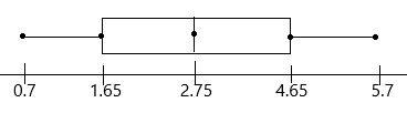
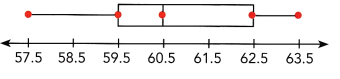
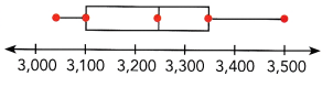
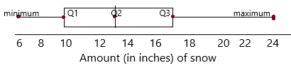
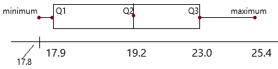
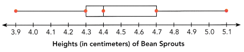
Refer to the box plot to answer the following.

The box plot summarizes the heights of bean sprouts, in centimeters.

Question 12.
Find the lower quartile, the median, and the upper quartile.
Answer:
Quartiles:
Quartiles mark each 25% of a set of data:
1. The first quartile Q₁ is the 25th percentile
2. The second quartile Q₂ is the 50th percentile
3. The third quartile Q₃ is the 75th percentile
Quartiles divide the entire set into four equal parts. So, there are three quartiles, first, second and third represented by Q₁, Q₂ and Q₃, respectively. Q₂ is nothing but the median, since it indicates the position of the item in the list and thus, is a positional average. To find quartiles of a group of data, we have to arrange the data in ascending order.
Suppose, Q₃ is the upper quartile is the median of the upper half of the data set. Whereas, Q₁ is the lower quartile and median of the lower half of the data set. Q₂ is the median.
The box plot summarizes five points. They are:
Lowest value;  Q1 (lower quartile); Q2 (median); Q3 (upper quartile); highest value.
Now observe the box plot and record the corresponding values.
Lowest value=3.9
Q1 (lower quartile)=4.3;
Q2 (median)=4.4;
Q3 (upper quartile)=4.7
Highest value=5.1

Question 13.
Calculate the range and the interquartile range.
Answer:
The range in statistics for a given data set is the difference between the highest and lowest values.
Range=maximum observation-minimum observation
how to find range:
To find the range in statistics, we need to arrange the given values or set of data or set of observations in ascending order. That means, firstly write the observations from the lowest to the highest value. Now, we need to use the formula to find the range of observations.
the data set: 3.9, 4.0, 4.1, 4.2, 4.3, 4.4, 4.5, 4.6, 4.7, 4.8, 4.9, 5.0, 5.1
Maximum value=5.1
Minimum value=3.9
range=5.1-3.9
range=1.2 cms
Interquartile range:
The interquartile range defines the difference between the third and the first quartile. Quartiles are the partitioned values that divide the whole series into 4 equal parts. So, there are 3 quartiles. First Quartile is denoted by Q₁ known as the lower quartile, the second Quartile is denoted by Q₂ and the third Quartile is denoted by Q₃ known as the upper quartile. Therefore, the interquartile range is equal to the upper quartile minus the lower quartile.
The difference between the upper and lower quartile is known as the interquartile range. The formula for the interquartile range is given below
Interquartile range = Upper Quartile – Lower Quartile = Q_­3 – Q1
where Q₁ is the first quartile and Q₃ is the third quartile of the series.
We know Q3=4.7; Q1=4.3 from this we can calculate IQR
IQR=Q3-Q1
IQR=4.7-4.3
IQR=0.4 cms

Question 14.
Math Journal Interpret what the range means in this context.
Answer:
The range in statistics for a given data set is the difference between the highest and lowest values.
Range=maximum observation-minimum observation
how to find range:
To find the range in statistics, we need to arrange the given values or set of data or set of observations in ascending order. That means, firstly write the observations from the lowest to the highest value. Now, we need to use the formula to find the range of observations.
the data set: 3.9, 4.0, 4.1, 4.2, 4.3, 4.4, 4.5, 4.6, 4.7, 4.8, 4.9, 5.0, 5.1
Maximum value=5.1
Minimum value=3.9
range=5.1-3.9
range=1.2 cms

Question 15.
Math Journal Interpret what the interquartile range means.
Answer:
The interquartile range defines the difference between the third and the first quartile. Quartiles are the partitioned values that divide the whole series into 4 equal parts. So, there are 3 quartiles. First Quartile is denoted by Q₁ known as the lower quartile, the second Quartile is denoted by Q₂ and the third Quartile is denoted by Q₃ known as the upper quartile. Therefore, the interquartile range is equal to the upper quartile minus the lower quartile.
The difference between the upper and lower quartile is known as the interquartile range. The formula for the interquartile range is given below
Interquartile range = Upper Quartile – Lower Quartile = Q_­3 – Q1
where Q₁ is the first quartile and Q₃ is the third quartile of the series.
We know Q3=4.7; Q1=4.3 from this we can calculate IQR
IQR=Q3-Q1
IQR=4.7-4.3
IQR=0.4 cms
Therefore, the spread of the middle 50% heights of the bean sprouts is 0.4 cms.

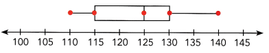
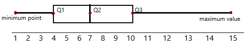
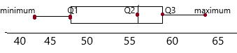
Use the box plot to answer the following.

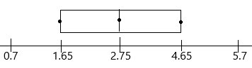
The box plot below summarizes the scores obtained by the contestants in a game.

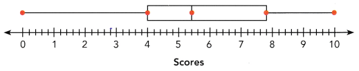
Question 16.
What are the greatest and the least scores?
Answer:
Quartiles:
Quartiles mark each 25% of a set of data:
1. The first quartile Q₁ is the 25th percentile
2. The second quartile Q₂ is the 50th percentile
3. The third quartile Q₃ is the 75th percentile
Quartiles divide the entire set into four equal parts. So, there are three quartiles, first, second and third represented by Q₁, Q₂ and Q₃, respectively. Q₂ is nothing but the median, since it indicates the position of the item in the list and thus, is a positional average. To find quartiles of a group of data, we have to arrange the data in ascending order.
Suppose, Q₃ is the upper quartile is the median of the upper half of the data set. Whereas, Q₁ is the lower quartile and median of the lower half of the data set. Q₂ is the median.
The box plot summarizes five points. They are:
Lowest value;  Q1 (lower quartile); Q2 (median); Q3 (upper quartile); highest value.
Now observe the box plot and record the corresponding values.
Here asked only greatest and least scores:
Greatest score=10
least score=0

Question 17.
Find the first, second, and third quartiles.
Answer:
Quartiles:
Quartiles mark each 25% of a set of data:
1. The first quartile Q₁ is the 25th percentile
2. The second quartile Q₂ is the 50th percentile
3. The third quartile Q₃ is the 75th percentile
Quartiles divide the entire set into four equal parts. So, there are three quartiles, first, second and third represented by Q₁, Q₂ and Q₃, respectively. Q₂ is nothing but the median, since it indicates the position of the item in the list and thus, is a positional average. To find quartiles of a group of data, we have to arrange the data in ascending order.
Suppose, Q₃ is the upper quartile is the median of the upper half of the data set. Whereas, Q₁ is the lower quartile and median of the lower half of the data set. Q₂ is the median.
The box plot summarizes five points. They are:
Lowest value;  Q1 (lower quartile); Q2 (median); Q3 (upper quartile); highest value.
Now observe the box plot and record the corresponding values.
Q1 (lower quartile)=4;
Q2 (median)=5.4;
Q3 (upper quartile)=7.8

Question 18.
If there are 160 contestants, how many scored 4 or more points?
Answer:
The number of contenstants=160
The number of members scored 4 or more=X
The maximum score is 10
X=160/10
X=16
Therefore, 16 members scored 4 or more points.

Problem Solving

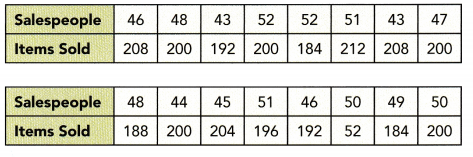
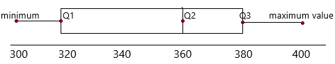
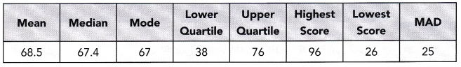
Use the statistics given ¡n the table to answer questions 19 to 21.

In a population of 200 students taking a science test, the following statistics for the test scores were compiled.

Question 19.
Math Journal By comparing the mean, the median, and the mode, what can you infer about the distribution of the test scores?
Answer:
The middle 50% of the science scores are moderately spread out from 38 to 76 and the mean is quite close to the median, making the distribution fairly symmetrical about the mean.

Question 20.
Math Journal By analyzing the statistics in the table, what can you infer about the variation of the scores?
Answer:
Inbetween the lowest and highest score the scores varied from one to one. The mean is quite close to the median.
Coming to quartiles there is a lot of variation from lower quartile to upper quartile.

Question 21.
Estimate the number of students who scored 76 or less.
Answer: 150 students.
The total number of students=200
76 or less means it can be 76 or 75, 74… up to 26 because it is the least number.
Suppose take 75% of 200
75*200/100
=150
Therefore, 150 students scored 76 or less.

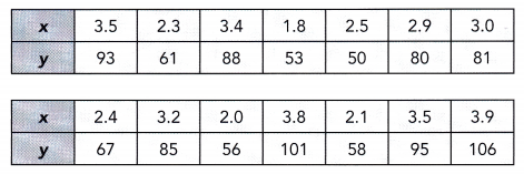
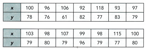
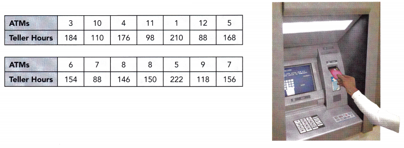
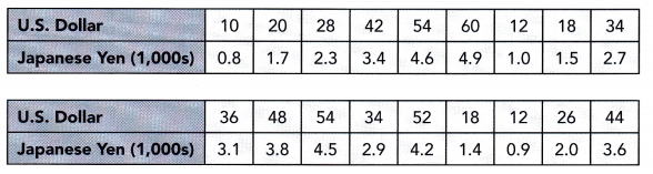
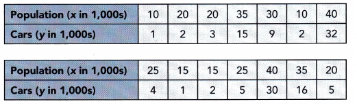
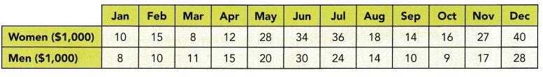
Use the data in the table to answer questions 22 to 27.

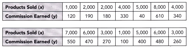
The table summarizes the monthly sales figures, in thousands of dollars, for the women’s and men’s clothing departments at a store. For instance, sales in the women’s department in January were $10,000.

Question 22.
Calculate the 5-point summary for each of the two departments.
Answer:
Quartiles mark each 25% of a set of data:
1. The first quartile Q₁ is the 25th percentile
2. The second quartile Q₂ is the 50th percentile
3. The third quartile Q₃ is the 75th percentile
Quartiles divide the entire set into four equal parts. So, there are three quartiles, first, second and third represented by Q₁, Q₂ and Q₃, respectively. Q₂ is nothing but the median, since it indicates the position of the item in the list and thus, is a positional average. To find quartiles of a group of data, we have to arrange the data in ascending order.
Suppose, Q₃ is the upper quartile is the median of the upper half of the data set. Whereas, Q₁ is the lower quartile and median of the lower half of the data set. Q₂ is the median.
The box plot summarizes five points. They are:
Lowest value;  Q1 (lower quartile); Q2 (median); Q3 (upper quartile); highest value.
Now observe the box plot and record the corresponding values.
The data set for women: 10, 15, 8, 12, 28, 34, 36, 18, 14, 16, 27, 40
The data set for men: 8, 10, 11, 15, 20, 30, 24, 14, 10, 9, 17, 28
Ascending order for women: 8, 10, 12, 14, 15, 16, 18, 27, 28, 34, 36, 40
Least point=8
Highest point=40
Q2=16+18/2
Q2=34/2
Q2=17
The first quartile Q₁ is the median of the lower half not including the value of Q₂. The third quartile Q₃ is the median of the upper half not including the value of Q₂.
Q1 data set: 8, 10, 12, 14, 15, 16
Q1=12+14/2
Q1=26/2
Q1=13
Q1 is the median of the lower half of the data.
Q3 data set: 18, 27, 28, 34, 36, 40
Q3=28+34/2
Q3=62/2
Q3=31
Q3 is the median of the upper half of the data.
Men’s department:
The data set for men: 8, 10, 11, 15, 20, 30, 24, 14, 10, 9, 17, 28
Ascending order: 8, 9, 10, 10, 11, 14, 15, 17, 20, 24, 28, 30
Lowest value=8
Highest value=30
Q2=14+15/2
Q2=29/2
Q2=14.5
Q1 data set: 8, 9, 10, 10, 11, 14
Q1=10+10/2
Q1=20/2
Q1=10
Q1 is the median of the lower half of the data.
Q3 data set: 15, 17, 20, 24, 28, 30
Q3=20+24/2
Q3=44/2
Q3=22
Q3 is the median of the upper half of the data.

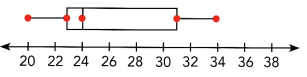
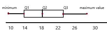
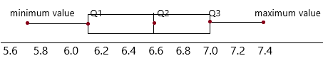
Question 23.
Using the same scale, draw 2 box plots, one for each department.
Answer:
When we display the data distribution in a standardized way using 5 summary – minimum, Q1 (First Quartile), median, Q3(third Quartile), and maximum, it is called a Box plot. It is also termed a box and whisker plot.
A box plot is a chart that shows data from a five-number summary including one of the measures of central tendency. It does not show the distribution in particular as much as a stem and leaf plot or histogram does. But it is primarily used to indicate a distribution is skewed or not and if there are potential unusual observations (also called outliers) present in the data set. Boxplots are also very beneficial when large numbers of data sets are involved or compared.

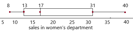
Question 24.
Math Journal By comparing the two box plots describe the sales performance of the two departments.
Answer:
By comparing two box plots, the sales are much quite closer to each other. There is not much difference between the women’s sales department and men’s sales department.

Question 25.
Calculate the mean sales figure for each of the two departments. Give your answers to the nearest dollar when you can.
Answer:
The data set for women: 10, 15, 8, 12, 28, 34, 36, 18, 14, 16, 27, 40
Mean=sum of observations/total number of observations.
Mean of women sale=10+15+8+12+28+34+36+18+14+16+27+40/12
Mean of women sale=258/12
mean of women sale=21.5
The data set for men: 8, 10, 11, 15, 20, 30, 24, 14, 10, 9, 17, 28
Mean of men’s sale=8+10+11+15+20+30+24+14+10+9+17+28/12
Mean of men’s sale=196/12
mean of men’s sale=16.3

Question 26.
Calculate the mean absolute deviation for each of the two departments. Give your answers to the nearest dollar.
Answer:
To understand Mean Absolute Deviation, let us split both the words and try to figure out their meaning. ‘Mean’ refers to the average of the observations and deviation implies departure or variation from a preset standard. When put together, we can define mean deviation as the mean distance of each observation from the mean of the data.
formula:
The ratio of the sum of all absolute values of deviation from central measure to the total number of observations.
M.A. D = (Σ Absolute Values of Deviation from Central Measure) / (Total Number of Observations)
Calculate MAD:
Steps to find the mean deviation from mean:
(i)Find the mean of the given observations.
(ii)Calculate the difference between each observation and the calculated mean
(iii)Evaluate the mean of the differences obtained in the second step.
This gives you the mean deviation from the mean.
The data set for women: 10, 15, 8, 12, 28, 34, 36, 18, 14, 16, 27, 40
Mean=sum of observations/total number of observations.
Mean of women sale=10+15+8+12+28+34+36+18+14+16+27+40/12
Mean of women sale=258/12
mean of women sale=21.5
|10-21.5|=11.5
|15-21.5|=6.5
|8-21.5|=13.5
|12-21.5|=9.5
|28-21.5|=6.5
|34-21.5|=12.5
|36-21.5|=14.5
|18-21.5|=3.5
|14-21.5|=7.5
|16-21.5|=5.5
|27-21.5|=5.5
|40-21.5|=18.5
now calculate mean for obtained differences:
MAD=11.5+6.5+13.5+9.5+6.5+12.5+14.5+3.5+7.5+5.5+5.5+18.5/12
MAD=115/12
MAD of women sale dapartment=9.58
The data set for men: 8, 10, 11, 15, 20, 30, 24, 14, 10, 9, 17, 28
Mean of men’s sale=8+10+11+15+20+30+24+14+10+9+17+28/12
Mean of men’s sale=196/12
mean of men’s sale=16.3
|8-16.3|=8.3
|10-16.3|=6.3
|11-16.3|=5.3
|15-16.3|=1.3
|20-16.3|=3.7
|30-16.3|=13.7
|24-16.3|=7.7
|14-16.3|=2.3
|10-16.3|=6.3
|9-16.3|=7.3
|17-16.3|=0.7
|28-16.3|=11.7
Now calculate the mean for obtained differences:
MAD=8.3+6.3+5.3+1.3+3.7+13.7+7.7+2.3+6.3+7.3+0.7+11.7/12
MAD=74.6/12
MAD of men’s sales department=6.21

Question 27.
Math Journal By comparing the means and the mean absolute deviations of the two clothing departments, what can you infer about their variability in sales?
Answer:
mean of women sale=21.5
mean of men’s sale=16.3
MAD of women sale dapartment=9.58
MAD of men’s sales department=6.21
MAD to mean ratio for women department:
9.58/21.5*100%
=44.6%
MAD to mean ratio for men’s department:
6.21/16.3*100%
=38.1%
By comparing all these, we can say the MAD to mean ratio for the women department is 44.6% and that of the men’s department is 38.1%. These two ratios show that the sales in the women department are slightly more varied than the sales in the men’s department.

Practice the problems of Math in Focus Grade 1 Workbook Answer Key Cumulative Review Chapters 10 to 13 to score better marks in the exam.

Math in Focus Grade 1 Cumulative Review Chapters 10 to 13 Answer Key

Concepts and Skills

Fill in the blanks.

Write heavier than, lighter than, or as heavy as.

Question 1.
The book is ___ the ball.
Answer: The book is heavier than the ball.

Question 2.
The doll is ___ the book.
Answer: The doll is lighter than the book.

Question 3.
The ball is ___ the doll.
Answer: The ball is heavier than the doll.

Fill in the blanks.

Question 4.

The ____ is lighter than the carrot.
The ____ is heavier than the carrot.
So, the tomato is lighter than the pineapple.
Answer:
The tomato is lighter than the carrot.
The pineapple is heavier than the carrot.

The picture graph shows the number of cars and trucks in a parking lot.

Fill in the blanks.

Question 5.
There are ____ more cars than trucks.
Answer: There are 2 more cars than trucks.

Question 6.
There are ____ cars and trucks in all.
Answer: There are cars 10 and trucks in all.

Question 7.
There are 2 fewer buses than cars. Draw to show the number of buses.
Answer:

Question 8.
Some cars leave the parking lot. The number of cars and trucks are now the same.
____ cars leave the parking lot.
Answer: 2 cars leave the parking lot.

Complete the tally chart using the data from the picture graph.

Question 9.

Answer:

Make a bar graph using the data from the tally chart.

Question 10.

Answer:

Fill in the blanks.

1 stands for 1 unit.

Question 11.
The weight of the box is __ units.
Answer: The weight of the box is 3 units.

Question 12.

Answer:

Fill in the blanks.

Question 13.
The weight of the toy shovel is about ___ toy bricks.
Answer: The weight of the toy shovel is about 10 toy bricks.

Question 14.
Order the objects from heaviest to lightest.

Answer:

First make tens.
Then count on.
Fill in the missing numbers.

Question 15.

Answer:

Question 16.

Answer:

Write the number.

Question 17.
twenty-five ____
Answer: 25

Question 18.
thirty ____
Answer: 30

Write the number in words.

Question 19.
37 _____
Answer: Thirty seven

Question 20.
40 ____
Answer: Fourty

Fill in the missing numbers.

Question 21.
1 + 20 = ____
Answer: 21

Question 22.
___ + 10 = 36
Answer: 26

Find the missing numbers.

Question 23.

38 = ___ tens ___ ones
Answer: 38 = 3 tens 8 ones

Look at the palce-value chart. Write the number it shows.

Question 24.

Answer:

Question 25.

Answer: 33

Circle the greater number.

Question 26.
25 or 17
Answer: 25 is greater than 17

Question 27.
26 or 29
Answer: 29 is greater than 26

Circle the number that is less.

Question 28.
10 or 29
Answer: 10

Question 29.
38 or 33
Answer: 33

Compare the numbers. Then fill in the blanks.

Question 30.
___ is the least.
Answer: 9 is the least.

Question 31.
____ is the greatest.
Answer: 35 is the greatest.

Question 32.
____ is less than 35 but greater than 16
Answer: 21 is less than 35 but greater than 16

Question 33.
Order the numbers from the least to greatest.

Answer: 9, 16, 21, 35

Complete each number pattern.

Question 34.
17, 20, 23, ___, ____, 32
Answer: 17, 20, 23, 26 , 29, 32
Add 3 to each number to get the next number.

Question 35.
28, ___, 36, 40
Answer: 28, 32, 36, 40
Add 4 to each number to get the next number

Fill in the blanks.

Question 36.
2 less than 25 is ____
Answer: 23

Question 37.
_______ is 3 more than 18.
Answer: 21

Question 38.
24 = _________ tens 4 ones
Answer: 2 tens 4 ones

Question 39.
18 = 1 ten _______ ones
Answer: 1 ten 8 ones

Add or subtract.

Question 40.
21 + 7 = ____
Answer: 28

Question 41.
24 + 10 = ___
Answer: 34

Question 42.
27 – 3 = ____
Answer: 24

Question 43.
38 – 15 = ____
Answer: 23

Question 44.
6 + 3 + 7 = ____
Answer: 16

Question 45.
9 + 8 + 5 = ___
Answer: 22

Question 46.

Answer:

Question 47.

Answer:

Question 48.

Answer:

Question 49.

Answer:

Question 50.

Answer:

Question 51.

Answer:

Question 52.

Answer:

Question 53.

Answer:

Problem Solving

Solve.

Question 54.
Jamal has 20 stamps. Michelle has 4- fewer stamps than Jamal. How many stamps does Michelle have?
Michelle has ____ stamps.
Answer:
Given,
Jamal has 20 stamps,
Michelle has 4 fewer stamps than Jamal,
By subtracting 4 from 20 we get 16,
Therefore, Michelle has 16 stamps.

Question 55.
Nate blows up 30 balloons for his birthday party. Nate blows up 6 fewer balloons than Miguel. How many balloons does Miguel blow up?
Miguel blows up ___ balloons.
Answer:
Given,
Nate blows up 30 balloons for his birthday party,
Nate blows up 6 fewer balloons than Miguel,
By adding 6 with 30 we get 36,
Therefore, Miguel blows up 36 balloons.

Practice the problems of Math in Focus Grade 1 Workbook Answer Key Chapter 14 Practice 1 Mental Addition to score better marks in the exam.

Math in Focus Grade 1 Chapter 14 Practice 1 Answer Key Mental Addition

Add mentally.
First add the ones.
Then add the ones to the tens.

Example

Question 1.
15 + 2 = ____
Answer: 17

Question 2.
12 + 4 = ____
Answer: 16

Question 3.
35 + 1 = ___
Answer: 36

Question 4.
23 + 5 = ____
Answer: 28

Question 5.
22 + 7 = ___
Answer: 29

Question 6.
31 + 8 = ___
Answer:

Question 7.
6 + 32 = ____
Answer:

Question 8.
5 + 34 = ____
Answer:

Add mentally.
First add the tens.
Then add the tens to the ones.

Example

Question 9.
18 + 10 = ____
Answer:

Question 10.
11 + 20 = ____
Answer: 31

Question 11.
12 + 10 = ____
Answer: 22

Question 12.
14 + 20 = ____
Answer: 34

Question 13.
16 + 10 = ____
Answer: 26

Question 14.
20 + 19 = ____
Answer: 39

Question 15.
10 + 17 = ___
Answer: 27

Question 16.
20 + 13 = ____
Answer: 33

Question 17.
10 + 14 = ____
Answer: 24

Question 18.
20 + 16 = ____
Answer: 36

Add mentally. Use doubles facts.

Example

Question 19.
4 + 5 = ____
Answer: 9
By doubling and adding 4 with 4 we get 8,
Then adding 8 with 1 we get 9.

Question 20.
7 + 8 = _____
Answer: 15
By doubling and adding 7 with 7 we get 14,
Then adding 14 with 1 we get 15.

Question 21.
5 + 6 = ___
Answer: 11
By doubling and adding 5 with 5 we get 10,
Then adding 10 with 1 we get 11.

Question 22.
8 + 9 = ____
Answer: 17
By doubling and adding 8 with 8 we get 16,
Then adding 16 with 1 we get 17.

Solve mentally. Fill in the blanks.

Question 23.

How many stickers will Emily have? ____
Answer:
Given,
Emily have 24 stickers and she needs 5 more,
By adding 24 with 5 we get 29,
Therefore, Emily will have 29 stickers in total.

Solve mentally. Fill in the blanks.

Question 24.

How many marbles are there in the box now? ____
Answer:
Given,
There are 18 marbles in the box,
And added 20 more marbles to it,
By adding 18 with 20 we get 38,
Therefore, there are 38 marbles in the box.

Question 25.

How many muffins does Baker Ross bake in all? _____
Answer:
Given,
There are 11 pecan muffins,
And 6 oat muffins,
By adding 11 with 6 we get 17,
Therefore, there are 17 muffins in total.

This handy Math in Focus Grade 7 Workbook Answer Key Chapter 9 Lesson 9.3 Understanding Box Plots and Mean Absolute Deviation detailed solutions for the textbook questions.

Math in Focus Grade 7 Course 2 B Chapter 9 Lesson 9.3 Answer Key Understanding Box Plots and Mean Absolute Deviation

Math in Focus Grade 7 Chapter 9 Lesson 9.3 Guided Practice Answer Key

Solve.

Question 1.
The box plot summarizes the age distribution of people in a play. State the lower quartile, the median, the upper quartile, the range, and the interquartile range.

Answer:
Quartiles divide the entire set into four equal parts. So, there are three quartiles, first, second and third represented by Q₁, Q₂ and Q₃, respectively. Q₂ is nothing but the median, since it indicates the position of the item in the list and thus, is a positional average. To find quartiles of a group of data, we have to arrange the data in ascending order.
In the median, we can measure the distribution with the help of lesser and higher quartile. Apart from mean and median, there are other measures in statistics, which can divide the data into specific equal parts. A median divides a series into two equal parts. We can partition values of a data set mainly into three different ways.
Quartiles formula:
Suppose, Q₃ is the upper quartile is the median of the upper half of the data set. Whereas, Q₁ is the lower quartile and median of the lower half of the data set. Q₂ is the median. Consider, we have n number of items in a data set. Then the quartiles are given by;
Q₁ = [(n+1)/4]th item
Q₂ = [(n+1)/2]th item
Q₃ = [3(n+1)/4]th item
In the above-given diagram:
quartiles are given that we need to find out.
The first dot represents the minimum value: 20
The second dot represents the Q1 (lower quartile):26
The third dot represents the Q2 (median):32
The fourth dot represents Q3 (upper quartile):34
The fifth dot represents the maximum value: 40

Construct a box plot.

Question 2.
The table shows the average monthly precipitation of Portland, Oregon, in inches. Draw a box plot of the average monthly rainfall and label it with the 5-point summary.

STEP 1: Arrange the data in ascending order.

STEP 2: Calculate the 5-point summary.
Q₁ = Q₂ = Q₃ =
Lower extreme value = Upper extreme value =

STEP 3: Draw a number line with a scale that covers both extreme values. Place a dot for each value from the 5-point summary.

STEP 4: Draw a box above the number line.

STEP 5: Draw the whiskers and label the box plot with the 5-point summary.
Answer:
The above-given data: 5.1, 4.2, 3.7, 2.6, 2.4, 1.6, 0.7, 0.9, 1.7, 2.9, 5.6, 5.7
Now arrange in ascending order:
0.7, 0.9, 1.6, 1.7, 2.4, 2.6, 2.9, 3.7, 4.2, 5.1, 5.6, 5.7
The minimum point is 0.7
the second quartile Q₂ is easy to find. It is the median of any data set and it divides an ordered data set into upper and lower halves.
Q2=2.6+2.9/2
Q2=5.5/2
Q2=2.75
The first quartile Q₁ is the median of the lower half not including the value of Q₂. The third quartile Q₃ is the median of the upper half not including the value of Q₂.
Q1 data set: 0.7, 0.9, 1.6, 1.7, 2.4, 2.6
Q1=1.6+1.7/2
Q1=3.3/2
Q1=1.65
Q1 is the median of the lower half of the data.
Q3 data set: 2.9, 3.7, 4.2, 5.1, 5.6, 5.7
Q3=4.2+5.1/2
Q3=9.3/2
Q3=4.65
Q3 is the median of the upper half of the data.
The maximum point is 5.7
Step 3:
Draw a number line with a scale that covers both extreme values. Place a dot for each value from the 5-point summary.

Step 4: Draw a box above the number line.

Step 5:
Draw the whiskers and label the box plot with the 5-point summary.

Average monthly rainfall.

Solve.

Question 3.
The scores on a math quiz are 20, 16, 13, 11, 19, 24, 22, 15, 17, and 13.
a) Find the mean absolute deviation.
STEP 1: Find the mean score.
Mean score =
STEP 2: Find the distance of each value from the mean.

STEP 3: Find the sum of the distances.
Sum =

STEP 4: Divide the sum by the number of data values to find the MAD.
MAD =
Answer:
Step 1: First we need to calculate mean
the given data: 20, 16, 13, 11, 19, 24, 22, 15, 17, and 13.
Mean=sum of observations/no.of observations
Mean=20+16+13+11+19+24+22+15+17+13/10
Mean=170/10
Mean=10
Step 2: Finding distance between each value
In statistics, the Mean Absolute Deviation (MAD) of the given data set value is defined as the average deviation between the mean and the data value. It describes the variation in the given data values. The procedure to find the mean absolute deviation is given below:
– Calculate the mean of the given data
– Determine the difference between each data value and the mean
– Now, take the absolute value of each obtained difference
– Finally, find the mean of these differences
|20-17|=3
|16-17|=1
|13-17|=4 Likewise, we need to subtract.

step 3: finding the sum of the above distances:
Sum=3+1+4+6+2+7+5+2+0+4
Sum=34
Step 4:
The formula for MAD:
The ratio of the sum of all absolute values of deviation from central measure to the total number of observations.
M.A. D = (Σ Absolute Values of Deviation from Central Measure) / (Total Number of Observations)
MAD=34/10
MAD=3.4

b) What does the mean absolute deviation tell you about this set of data?
Answer:  On average, the data values are 3.4 units from the mean.
This gives us an idea about the deviation of the observations from the measure of central tendency.
Thus we can conclude that,
M.A.D=$\frac{\sum Absolute values of Deviation from cental measure/Total Number of observations.}{}$

Although to calculate mean absolute deviation, any measure of central tendency can be used out generally mean and median are the most common ones.
Technology Activity

Materials

• spreadsheet software
• two sets of 10 data values

USE SPREADSHEET SOFTWARE TO FIND MEAN ABSOLUTE DEVIATION

Work in pairs.

STEP 1: Enter 10 data values in one row of cells.

STEP 2: Choose a cell in a later row for the mean.

STEP 3: Use the spreadsheet software’s function for finding the mean to find the mean of the 10 data values.
See the screen shot below.

STEP 4: Choose a cell in the next row for the mean absolute deviation.

STEP 5: Use the spreadsheet software’s function for finding the mean absolute deviation to find the MAD of the data values.

STEP 6: Explain what the MAD tells you about the data.

STEP 7: Enter a second set of data values and repeat STEP 1 to STEP 6.

Math Journal Compare the two sets of data. Are the data values in each set clustered around the mean, or more spread out? Then compare the mean absolute deviations for the two sets of data. What do you observe?
Answer:

Math in Focus Course 2B Practice 9.3 Answer Key

State Q₁, Q₂, Q₃ the lower extreme, and the upper extreme values shown in the box plots. Then calculate the interquartile range.

Question 1.

Answer:
Quartiles divide the entire set into four equal parts. So, there are three quartiles, first, second and third represented by Q₁, Q₂ and Q₃, respectively. Q₂ is nothing but the median, since it indicates the position of the item in the list and thus, is a positional average. To find quartiles of a group of data, we have to arrange the data in ascending order.
In the median, we can measure the distribution with the help of lesser and higher quartile. Apart from mean and median, there are other measures in statistics, which can divide the data into specific equal parts. A median divides a series into two equal parts. We can partition values of a data set mainly into three different ways.
Quartiles formula:
Suppose, Q₃ is the upper quartile is the median of the upper half of the data set. Whereas, Q₁ is the lower quartile and median of the lower half of the data set. Q₂ is the median. Consider, we have n number of items in a data set. Then the quartiles are given by;
Q₁ = [(n+1)/4]th item
Q₂ = [(n+1)/2]th item
Q₃ = [3(n+1)/4]th item
In the above-given diagram:
quartiles are given that we need to find out.
The first dot represents the minimum value: 57.5
The second dot represents the Q1 (lower quartile):59.5
The third dot represents the Q2 (median):60.5
The fourth dot represents Q3 (upper quartile):62.5
The fifth dot represents the maximum value: 63.5

Question 2.

Answer:
Quartiles divide the entire set into four equal parts. So, there are three quartiles, first, second and third represented by Q₁, Q₂ and Q₃, respectively. Q₂ is nothing but the median, since it indicates the position of the item in the list and thus, is a positional average. To find quartiles of a group of data, we have to arrange the data in ascending order.
In the median, we can measure the distribution with the help of lesser and higher quartile. Apart from mean and median, there are other measures in statistics, which can divide the data into specific equal parts. A median divides a series into two equal parts. We can partition values of a data set mainly into three different ways.
Quartiles formula:
Suppose, Q₃ is the upper quartile is the median of the upper half of the data set. Whereas, Q₁ is the lower quartile and median of the lower half of the data set. Q₂ is the median. Consider, we have n number of items in a data set. Then the quartiles are given by;
Q₁ = [(n+1)/4]th item
Q₂ = [(n+1)/2]th item
Q₃ = [3(n+1)/4]th item
In the above-given diagram:
quartiles are given that we need to find out.
The first dot represents the minimum value: 110
The second dot represents the Q1 (lower quartile):115
The third dot represents the Q2 (median):125
The fourth dot represents Q3 (upper quartile):130
The fifth dot represents the maximum value: 140

Question 3.

Answer:
Quartiles divide the entire set into four equal parts. So, there are three quartiles, first, second and third represented by Q₁, Q₂ and Q₃, respectively. Q₂ is nothing but the median, since it indicates the position of the item in the list and thus, is a positional average. To find quartiles of a group of data, we have to arrange the data in ascending order.
In the median, we can measure the distribution with the help of lesser and higher quartile. Apart from mean and median, there are other measures in statistics, which can divide the data into specific equal parts. A median divides a series into two equal parts. We can partition values of a data set mainly into three different ways.
Quartiles formula:
Suppose, Q₃ is the upper quartile is the median of the upper half of the data set. Whereas, Q₁ is the lower quartile and median of the lower half of the data set. Q₂ is the median. Consider, we have n number of items in a data set. Then the quartiles are given by;
Q₁ = [(n+1)/4]th item
Q₂ = [(n+1)/2]th item
Q₃ = [3(n+1)/4]th item
In the above-given diagram:
quartiles are given that we need to find out.
The first dot represents the minimum value: 20
The second dot represents the Q1 (lower quartile):23
The third dot represents the Q2 (median):24
The fourth dot represents Q3 (upper quartile):31
The fifth dot represents the maximum value: 34

Question 4.

Answer:
Quartiles divide the entire set into four equal parts. So, there are three quartiles, first, second and third represented by Q₁, Q₂ and Q₃, respectively. Q₂ is nothing but the median, since it indicates the position of the item in the list and thus, is a positional average. To find quartiles of a group of data, we have to arrange the data in ascending order.
In the median, we can measure the distribution with the help of lesser and higher quartile. Apart from mean and median, there are other measures in statistics, which can divide the data into specific equal parts. A median divides a series into two equal parts. We can partition values of a data set mainly into three different ways.
Quartiles formula:
Suppose, Q₃ is the upper quartile is the median of the upper half of the data set. Whereas, Q₁ is the lower quartile and median of the lower half of the data set. Q₂ is the median. Consider, we have n number of items in a data set. Then the quartiles are given by;
Q₁ = [(n+1)/4]th item
Q₂ = [(n+1)/2]th item
Q₃ = [3(n+1)/4]th item
In the above-given diagram:
quartiles are given that we need to find out.
The first dot represents the minimum value: 3,050
The second dot represents the Q1 (lower quartile):3,100
The third dot represents the Q2 (median):3,250
The fourth dot represents Q3 (upper quartile):3,350
The fifth dot represents the maximum value: 3,500

Draw a box plot for the given 5-point summary. Include a numeric scale for the number line. Label the box plot with the 5-point summary.

Question 5.
Q₁ = 4, Q₂ = 7, Q₃ = 10, lower extreme value = 1, upper extreme value = 15
Answer:
A box and whisker plot is a graph that exhibits data from a five-number summary, including one of the measures of central tendency. It does not display the distribution as accurately as a stem and leaf plot or histogram does. But, it is principally used to show whether a distribution is skewed or not and if there are potential unusual observations present in the data set, which are also called outliers. Boxplots are also very useful when huge numbers of data collections are involved or compared. Since the centre, spread and overall range are instantly apparent, using these boxplots the arrangements can be matched easily. A box and whisker plot is a way of compiling a set of data outlined on an interval scale. It is also used for descriptive data interpretation.
Elements of a Box and Whisker Plot:
The elements required to construct a box and whisker plot outliers are given below.
The minimum value (Q₀ or 0th percentile)
The first quartile (Q₁ or 25th percentile)
Median (Q₂ or 50th percentile)
Third quartile (Q₃ or 75th percentile)
The maximum value (Q₄ or 100th percentile)
– When we plot a graph for the box plot, we outline a box from the first quartile to the third quartile. A vertical line that goes through the box is the median. The whiskers (small lines) go from each quartile towards the minimum or maximum value, as shown in the figure below.

Question 6.
Q₁ = 14, Q₂ = 18, Q₃ = 23, lower extreme value = 10, upper extreme value = 28
Answer:
A box and whisker plot is a graph that exhibits data from a five-number summary, including one of the measures of central tendency. It does not display the distribution as accurately as a stem and leaf plot or histogram does. But, it is principally used to show whether a distribution is skewed or not and if there are potential unusual observations present in the data set, which are also called outliers. Boxplots are also very useful when huge numbers of data collections are involved or compared. Since the centre, spread and overall range are instantly apparent, using these boxplots the arrangements can be matched easily. A box and whisker plot is a way of compiling a set of data outlined on an interval scale. It is also used for descriptive data interpretation.
Elements of a Box and Whisker Plot:
The elements required to construct a box and whisker plot outliers are given below.
The minimum value (Q₀ or 0th percentile)
The first quartile (Q₁ or 25th percentile)
Median (Q₂ or 50th percentile)
Third quartile (Q₃ or 75th percentile)
The maximum value (Q₄ or 100th percentile)
– When we plot a graph for the box plot, we outline a box from the first quartile to the third quartile. A vertical line that goes through the box is the median. The whiskers (small lines) go from each quartile towards the minimum or maximum value, as shown in the figure below.

Question 7.
Q₁ = 6.1, Q₂ = 6.6, Q₃ = 7.0, lower extreme value = 5.7, upper extreme value = 7.4
Answer:
A box and whisker plot is a graph that exhibits data from a five-number summary, including one of the measures of central tendency. It does not display the distribution as accurately as a stem and leaf plot or histogram does. But, it is principally used to show whether a distribution is skewed or not and if there are potential unusual observations present in the data set, which are also called outliers. Boxplots are also very useful when huge numbers of data collections are involved or compared. Since the centre, spread and overall range are instantly apparent, using these boxplots the arrangements can be matched easily. A box and whisker plot is a way of compiling a set of data outlined on an interval scale. It is also used for descriptive data interpretation.
Elements of a Box and Whisker Plot:
The elements required to construct a box and whisker plot outliers are given below.
The minimum value (Q₀ or 0th percentile)
The first quartile (Q₁ or 25th percentile)
Median (Q₂ or 50th percentile)
Third quartile (Q₃ or 75th percentile)
The maximum value (Q₄ or 100th percentile)
– When we plot a graph for the box plot, we outline a box from the first quartile to the third quartile. A vertical line that goes through the box is the median. The whiskers (small lines) go from each quartile towards the minimum or maximum value, as shown in the figure below.

Question 8.
Q₁ = 320, Q₂ = 360, Q₃ = 380, lower extreme value = 300, upper extreme value = 400
Answer:
A box and whisker plot is a graph that exhibits data from a five-number summary, including one of the measures of central tendency. It does not display the distribution as accurately as a stem and leaf plot or histogram does. But, it is principally used to show whether a distribution is skewed or not and if there are potential unusual observations present in the data set, which are also called outliers. Boxplots are also very useful when huge numbers of data collections are involved or compared. Since the centre, spread and overall range are instantly apparent, using these boxplots the arrangements can be matched easily. A box and whisker plot is a way of compiling a set of data outlined on an interval scale. It is also used for descriptive data interpretation.
Elements of a Box and Whisker Plot:
The elements required to construct a box and whisker plot outliers are given below.
The minimum value (Q₀ or 0th percentile)
The first quartile (Q₁ or 25th percentile)
Median (Q₂ or 50th percentile)
Third quartile (Q₃ or 75th percentile)
The maximum value (Q₄ or 100th percentile)
– When we plot a graph for the box plot, we outline a box from the first quartile to the third quartile. A vertical line that goes through the box is the median. The whiskers (small lines) go from each quartile towards the minimum or maximum value, as shown in the figure below.

Calculate the mean absolute deviation. Round your answers to 3 significant digits when you can.

Question 9.
2, 2, 5, 3, 9, 6,10, 4, 7, 5
Answer:
We begin with the definition of the mean absolute deviation, which is also referred to as the average absolute deviation. It may make more sense to consider this formula as a process, or series of steps, that we can use to obtain our statistic.
1. We start with an average, of a data set, which we will denote by m.
2. Next, we find how much each of the data values deviates from m. This means that we take the difference between each of the data values and m.
3. After this, we take the absolute value of each of the differences from the previous step. In other words, we drop any negative signs for any of the differences. The reason for doing this is that there are positive and negative deviations from m. If we do not figure out a way to eliminate the negative signs, all of the deviations will cancel one another out if we add them together.
4. Now we add together all of these absolute values.
5. Finally, we divide this sum by n, which is the total number of data values. The result is the mean absolute deviation.
The above-given data: 2, 2, 5, 3, 9, 6,10, 4, 7, 5
First find out the Mean:
Mean=sum of observations/number of observations
Mean=2+2+5+3+9+6+10+4+7+5/10
Mean=53/10
Mean=5.3
– Determine the difference between each data value and the mean
|2-5.3|=3.3
|2-5.3|=3.3
|5-5.3|=0.3
|3-5.3|=2.3
|9-5.3|=3.7
|6-5.3|=0.7
|10-5.3|=4.7
|4-5.3|=1.3
|7-5.3|=1.7
|5-5.3|=0.3
– Now, take the absolute value of each obtained difference
The obtained values are 3.3, 3.3, 0.3, 2.3, 3.7, 0.7, 4.7, 1.3, 1.7, 0.3
– Finally, find the mean of these differences
The formula for MAD:
The ratio of the sum of all absolute values of deviation from central measure to the total number of observations.
M.A. D = (Σ Absolute Values of Deviation from Central Measure) / (Total Number of Observations)
MAD=3.3+ 3.3+0.3+ 2.3+ 3.7+0.7+ 4.7+1.3+1.7+0.3/10
MAD=21.6/10
MAD=2.16

Question 10.
58, 62, 45, 39, 40, 60, 67
Answer:
We begin with the definition of the mean absolute deviation, which is also referred to as the average absolute deviation. It may make more sense to consider this formula as a process, or series of steps, that we can use to obtain our statistic.
1. We start with an average, of a data set, which we will denote by m.
2. Next, we find how much each of the data values deviates from m. This means that we take the difference between each of the data values and m.
3. After this, we take the absolute value of each of the differences from the previous step. In other words, we drop any negative signs for any of the differences. The reason for doing this is that there are positive and negative deviations from m. If we do not figure out a way to eliminate the negative signs, all of the deviations will cancel one another out if we add them together.
4. Now we add together all of these absolute values.
5. Finally, we divide this sum by n, which is the total number of data values. The result is the mean absolute deviation.
The above-given data: 58, 62, 45, 39, 40, 60, 67
First find out the Mean:
Mean=58+62+45+39+40+60+67/7
Mean=371/7
Mean=53
– Determine the difference between each data value and the mean
|58-53|=5
|62-53|=9
|45-53|=8
|39-53|=14
|40-53|=13
|60-53|=7
|67-53|=14
– Now, take the absolute value of each obtained difference
The obtained difference values: 5, 9, 8, 14, 13, 7, 14
– Finally, find the mean of these differences
MAD=5+9+8+14+13+7+14/7
MAD=70/7
MAD=7

Question 11.
43.4, 30.5, 20.0, 23.6, 34.5, 36.9, 11.7, 40.2
Answer:
We begin with the definition of the mean absolute deviation, which is also referred to as the average absolute deviation. It may make more sense to consider this formula as a process, or series of steps, that we can use to obtain our statistic.
1. We start with an average, of a data set, which we will denote by m.
2. Next, we find how much each of the data values deviates from m. This means that we take the difference between each of the data values and m.
3. After this, we take the absolute value of each of the differences from the previous step. In other words, we drop any negative signs for any of the differences. The reason for doing this is that there are positive and negative deviations from m. If we do not figure out a way to eliminate the negative signs, all of the deviations will cancel one another out if we add them together.
4. Now we add together all of these absolute values.
5. Finally, we divide this sum by n, which is the total number of data values. The result is the mean absolute deviation.
The above-given data: 43.4, 30.5, 20.0, 23.6, 34.5, 36.9, 11.7, 40.2
First find out the Mean:
Mean=43.4+30.5+20.0+23.6+34.5+36.9+11.7+40.2/8
Mean=240.8/8
Mean=30.1
– Determine the difference between each data value and the mean
|43.4-30.1|=13.3
|30.5-30.1|=0.4
|20.0-30.1|=10.1
|23.6-30.1|=6.5
|34.5-30.1|=4.4
|36.9-30.1|=6.8
|11.7-30.1|=18.4
|40.2-30.1|=10.1
– Now, take the absolute value of each obtained difference
The obtained difference values: 13.3, 0.4, 10.1, 6.5, 4.4, 6.8, 18.4, 10.1
– Finally, find the mean of these differences
MAD=13.3+0.4+10.1+6.5+4.4+6.8+18.4+10.1/8
MAD=70/8
MAD=8.75

Question 12.
1.15, 1.16, 1.25, 1.22, 1.36, 1.38, 1.49, 1.22, 1.11
Answer:
We begin with the definition of the mean absolute deviation, which is also referred to as the average absolute deviation. It may make more sense to consider this formula as a process, or series of steps, that we can use to obtain our statistic.
1. We start with an average, of a data set, which we will denote by m.
2. Next, we find how much each of the data values deviates from m. This means that we take the difference between each of the data values and m.
3. After this, we take the absolute value of each of the differences from the previous step. In other words, we drop any negative signs for any of the differences. The reason for doing this is that there are positive and negative deviations from m. If we do not figure out a way to eliminate the negative signs, all of the deviations will cancel one another out if we add them together.
4. Now we add together all of these absolute values.
5. Finally, we divide this sum by n, which is the total number of data values. The result is the mean absolute deviation.
The above-given data: 1.15, 1.16, 1.25, 1.22, 1.36, 1.38, 1.49, 1.22, 1.11
First find out the Mean:
Mean=1.15+1.16+1.25+1.22+1.36+1.38+1.49+1.22+1.11/9
Mean=11.34/9
Mean=1.26
– Determine the difference between each data value and the mean
|1.15-1.26|=0.11
|1.16-1.26|=0.1
|1.25-1.26|=0.01
|1.22-1.26|=0.04
|1.36-1.26|=0.1
|1.38-1.26|=0.12
|1.49-1.26|=0.23
|1.22-1.26|=0.04
|1.11-1.26|=0.15
– Now, take the absolute value of each obtained difference
The obtained difference values: 0.11, 0.1, 0.01, 0.04, 0.1, 0.12, 0.23, 0.04, 0.15
– Finally, find the mean of these differences
MAD=0.11+0.1+0.01+0.04+0.1+0.12+0.23+0.04+0.15/9
MAD=0.9/9
MAD=0.1

Use the data in the table for the following questions.

The table shows the masses, in grams, of a dozen eggs.

Question 13.
Calculate Q₁, Q₂, and Q₃.
Answer:
The given data: 57, 53, 62, 45, 56, 56, 63, 61, 50, 44, 43, 58
How to calculate quartiles:
1. Order your data set from lowest to highest values
2. Find the median. This is the second quartile Q₂.
3. At Q₂ split the ordered data set into two halves.
4. The lower quartile Q₁ is the median of the lower half of the data.
5. The upper quartile Q₃ is the median of the upper half of the data.
Now arrange the data set in ascending order:
43, 44, 45, 50, 53, 56, 56, 57, 58, 61, 62, 63
Now find the median:
Q2=56+56/2
Q2=112/2
Q2=56
Now find Q1: The lower quartile Q₁ is the median of the lower half of the data.
Q1 data set: 43, 44, 45, 50, 53, 56
Q1=45+50/2
Q1=95/2
Q1=47.5
Q₁ is the median of the lower half of the data.
Now find Q3: The upper quartile Q₃ is the median of the upper half of the data.
Q3 data set: 56, 57, 58, 61, 62, 63
Q3=58+61/2
Q3=119/2
Q3=59.5
Q₃ is the median of the upper half of the data.

Question 14.
Draw a box plot of the masses of the eggs.
Answer:
the above quartiles we got are
Q1=47.5, Q2=56, Q3=59.5, lower value=43, higher value=63
A box and whisker plot is a graph that exhibits data from a five-number summary, including one of the measures of central tendency. It does not display the distribution as accurately as a stem and leaf plot or histogram does. But, it is principally used to show whether a distribution is skewed or not and if there are potential unusual observations present in the data set, which are also called outliers. Boxplots are also very useful when huge numbers of data collections are involved or compared. Since the centre, spread and overall range are instantly apparent, using these boxplots the arrangements can be matched easily. A box and whisker plot is a way of compiling a set of data outlined on an interval scale. It is also used for descriptive data interpretation.
Elements of a Box and Whisker Plot:
The elements required to construct a box and whisker plot outliers are given below.
The minimum value (Q₀ or 0th percentile)
The first quartile (Q₁ or 25th percentile)
Median (Q₂ or 50th percentile)
Third quartile (Q₃ or 75th percentile)
The maximum value (Q₄ or 100th percentile)
– When we plot a graph for the box plot, we outline a box from the first quartile to the third quartile. A vertical line that goes through the box is the median. The whiskers (small lines) go from each quartile towards the minimum or maximum value, as shown in the figure below.

Question 15.
Calculate the mean absolute deviation of the masses of the eggs. Round to the nearest hundredth.
Answer:
We begin with the definition of the mean absolute deviation, which is also referred to as the average absolute deviation. It may make more sense to consider this formula as a process, or series of steps, that we can use to obtain our statistic.
1. We start with an average, of a data set, which we will denote by m.
2. Next, we find how much each of the data values deviates from m. This means that we take the difference between each of the data values and m.
3. After this, we take the absolute value of each of the differences from the previous step. In other words, we drop any negative signs for any of the differences. The reason for doing this is that there are positive and negative deviations from m. If we do not figure out a way to eliminate the negative signs, all of the deviations will cancel one another out if we add them together.
4. Now we add together all of these absolute values.
5. Finally, we divide this sum by n, which is the total number of data values. The result is the mean absolute deviation.
The above-given data: 43, 44, 45, 50, 53, 56, 56, 57, 58, 61, 62, 63
First find out the Mean:
Mean=43+44+45+50+53+56+56+57+58+61+61+63/12
Mean=647/12
Mean=53.9
Mean=54 (rounded to nearest number)
– Determine the difference between each data value and the mean
|43-54|=11
|44-54|=10
|45-54|=9
|50-54|=4
|53-54|=1
|56-54|=2
|56-54|=2
|57-54|=3
|58-54|=4
|61-54|=7
|61-54|=7
|63-54|=9
– Now, take the absolute value of each obtained difference
The obtained difference values: 11, 10, 9, 4, 1, 2, 2, 3, 4, 7, 7, 9
– Finally, find the mean of these differences
MAD=11+10+9+4+1+2+2+3+4+7+7+9/12
MAD=69/12
MAD=5.75

Use the information to answer the following questions.

The map shows the amounts of snow, in inches, that fell in different parts of Minnesota during one week in winter.

Question 16.
Calculate Q₁, Q₂, and Q₃.
Answer:
The given data: 13, 6, 8, 15, 9, 18, 18, 20, 24, 16, 11, 10, 13, 15, 10, 12
How to calculate quartiles:
1. Order your data set from lowest to highest values
2. Find the median. This is the second quartile Q₂.
3. At Q₂ split the ordered data set into two halves.
4. The lower quartile Q₁ is the median of the lower half of the data.
5. The upper quartile Q₃ is the median of the upper half of the data.
Now arrange the data set in ascending order:
6, 8, 9, 10, 10, 11, 12, 13, 13, 15, 15, 16, 18, 18, 20, 24
Now find the median:
Q2=13+13/2
Q2=26/2
Q2=13
Now find Q1: The lower quartile Q₁ is the median of the lower half of the data.
Q1 data set: 6, 8, 9, 10, 10, 11, 12, 13
Q1=10+10/2
Q1=20/2
Q1=10
Q₁ is the median of the lower half of the data.
Now find Q3: The upper quartile Q₃ is the median of the upper half of the data.
Q3 data set: 13, 15, 15, 16, 18, 18, 20, 24
Q3=16+18/2
Q3=34/2
Q3=17
Q₃ is the median of the upper half of the data.

Question 17.
Draw a box plot of the snow amounts.
Answer:
the above quartiles we got are:
Q1=10, Q2=13, Q3=17, lowest value=6, highest value=24
A box and whisker plot is a graph that exhibits data from a five-number summary, including one of the measures of central tendency. It does not display the distribution as accurately as a stem and leaf plot or histogram does. But, it is principally used to show whether a distribution is skewed or not and if there are potential unusual observations present in the data set, which are also called outliers. Boxplots are also very useful when huge numbers of data collections are involved or compared. Since the centre, spread and overall range are instantly apparent, using these boxplots the arrangements can be matched easily. A box and whisker plot is a way of compiling a set of data outlined on an interval scale. It is also used for descriptive data interpretation.
Elements of a Box and Whisker Plot:
The elements required to construct a box and whisker plot outliers are given below.
The minimum value (Q₀ or 0th percentile)
The first quartile (Q₁ or 25th percentile)
Median (Q₂ or 50th percentile)
Third quartile (Q₃ or 75th percentile)
The maximum value (Q₄ or 100th percentile)
– When we plot a graph for the box plot, we outline a box from the first quartile to the third quartile. A vertical line that goes through the box is the median. The whiskers (small lines) go from each quartile towards the minimum or maximum value, as shown in the figure below.

Question 18.
Calculate the mean absolute deviation of the snow amounts. Round your answer to the nearest inch.
Answer:
We begin with the definition of the mean absolute deviation, which is also referred to as the average absolute deviation. It may make more sense to consider this formula as a process, or series of steps, that we can use to obtain our statistic.
1. We start with an average, of a data set, which we will denote by m.
2. Next, we find how much each of the data values deviates from m. This means that we take the difference between each of the data values and m.
3. After this, we take the absolute value of each of the differences from the previous step. In other words, we drop any negative signs for any of the differences. The reason for doing this is that there are positive and negative deviations from m. If we do not figure out a way to eliminate the negative signs, all of the deviations will cancel one another out if we add them together.
4. Now we add together all of these absolute values.
5. Finally, we divide this sum by n, which is the total number of data values. The result is the mean absolute deviation.
The above-given data:
First find out the Mean: 6, 8, 9, 10, 10, 11, 12, 13, 13, 15, 15, 16, 18, 18, 20, 24
Mean=sum of observations/number of observations
Mean=6+8+9+10+10+11+12+13+13+15+15+16+18+18+20+24/16
Mean=218/16
Mean=13.265
Mean=14(nearest inch)
– Determine the difference between each data value and the mean
|6-14|=8
|8-14|=6
|9-14|=5
|10-14|=4
|10-14|=4
|11-14|=3
|12-14|=2
|13-14|=1
|13-14|=1
|15-14|=1
|15-14|=1
|16-14|=2
|18-14|=4
|18-14|=4
|20-14|=6
|24-14|=10
– Now, take the absolute value of each obtained difference
The obtained values are 8, 6, 6, 4, 4, 3, 2, 1, 1, 1, 1, 2, 4, 4, 6, 10
– Finally, find the mean of these differences
The formula for MAD:
The ratio of the sum of all absolute values of deviation from central measure to the total number of observations.
M.A. D = (Σ Absolute Values of Deviation from Central Measure) / (Total Number of Observations)
MAD=8+6+6+4+4+3+2+1+1+1+1+2+4+4+6+10/16
MAD=53/16
MAD=3.3

Use the data in the table for questions 19 and 20.

The table shows the heights, in centimeters, of 5 peanut plants.

Question 19.
Draw a box plot of the heights of the peanut plants.
Answer:
The given data: 17.8, 25.4, 20.6, 18.0, 19.2
A box and whisker plot is a graph that exhibits data from a five-number summary, including one of the measures of central tendency. It does not display the distribution as accurately as a stem and leaf plot or histogram does. But, it is principally used to show whether a distribution is skewed or not and if there are potential unusual observations present in the data set, which are also called outliers. Boxplots are also very useful when huge numbers of data collections are involved or compared. Since the centre, spread and overall range are instantly apparent, using these boxplots the arrangements can be matched easily. A box and whisker plot is a way of compiling a set of data outlined on an interval scale. It is also used for descriptive data interpretation.
Elements of a Box and Whisker Plot:
The elements required to construct a box and whisker plot outliers are given below.
The minimum value (Q₀ or 0th percentile)
The first quartile (Q₁ or 25th percentile)
Median (Q₂ or 50th percentile)
Third quartile (Q₃ or 75th percentile)
The maximum value (Q₄ or 100th percentile)
– When we plot a graph for the box plot, we outline a box from the first quartile to the third quartile. A vertical line that goes through the box is the median. The whiskers (small lines) go from each quartile towards the minimum or maximum value, as shown in the figure below.

Question 20.
Calculate the mean absolute deviation of the heights of the peanut plants.
Answer:
We begin with the definition of the mean absolute deviation, which is also referred to as the average absolute deviation. It may make more sense to consider this formula as a process, or series of steps, that we can use to obtain our statistic.
1. We start with an average, of a data set, which we will denote by m.
2. Next, we find how much each of the data values deviates from m. This means that we take the difference between each of the data values and m.
3. After this, we take the absolute value of each of the differences from the previous step. In other words, we drop any negative signs for any of the differences. The reason for doing this is that there are positive and negative deviations from m. If we do not figure out a way to eliminate the negative signs, all of the deviations will cancel one another out if we add them together.
4. Now we add together all of these absolute values.
5. Finally, we divide this sum by n, which is the total number of data values. The result is the mean absolute deviation.
The above-given data:
First find out the Mean: The given data: 17.8, 25.4, 20.6, 18.0, 19.2
Mean=sum of observations/number of observations
Mean=17.8+25.4+20.6+18.0+19.2/5
Mean=101/5
Mean=20.2
– Determine the difference between each data value and the mean
|17.8-20.2|=2.4
|25.4-20.2|=5.2
|20.6-20.2|=0.4
|18.0-20.2|=2.2
|19.2-20.2|=1
– Now, take the absolute value of each obtained difference
The obtained values are 2.4+5.2+0.4+2.2+1
– Finally, find the mean of these differences
The formula for MAD:
The ratio of the sum of all absolute values of deviation from central measure to the total number of observations.
M.A. D = (Σ Absolute Values of Deviation from Central Measure) / (Total Number of Observations)
MAD=2.4+5.2+0.4+2.2+1/5
MAD=11.2/5
MAD=2.24

Solve.

Question 21.
Math journal Compare the box plot and the mean absolute deviation. Which one is a better measure of variation? State your reason.
Answer:
Mean absolute deviation is a better measure of variation. A box plot is not meaningful with only 5 data values.

Question 22.
Math Journal Describe a situation for which you think a box plot would be useful for measuring variation.
Answer:
You need to have information on the variability or dispersion of the data. A boxplot is a graph that gives you a good indication of how the values in the data are spread out. Although boxplots may seem primitive in comparison to a histogram or density plot, they have the advantage of taking up less space, which is useful when comparing distributions between many groups or datasets.

Question 23.
Math journal Describe a situation for which you think the mean absolute deviation would be useful for measuring variation.
Answer:
the mean absolute deviation is most useful when you are interested in how data are spread from the mean.

This handy Math in Focus Grade 7 Workbook Answer Key Chapter 9 Lesson 9.2 Stem-and-Leaf Plots detailed solutions for the textbook questions.

Math in Focus Grade 7 Course 2 B Chapter 9 Lesson 9.2 Answer Key Stem-and-Leaf Plots

Math in Focus Grade 7 Chapter 9 Lesson 9.2 Guided Practice Answer Key

Display data in a stem-and-leaf plot.

Question 1.
The data show the math quiz scores for 15 students. Display the data in a stem-and-leaf plot.

STEP 1: Identify the least and greatest values, and identify the stems.
STEP 2: Place a leaf on the plot for each item of data.
STEP 3: Arrange the leaves in ascending order for each number on the stem.
STEP 4: Write a title and a key for the stem-and-leaf plot.
Answer:
Step 1: Least value:8; greatest value:44; stems:0, 1, 2, 3, 4
Step 2:  Constructing leaf for item of data

Step 3: Now arrange in ascending order

Step 4: Write the title, Remember, a Stem and Leaf plot can have multiple sets of leaves.
0|8 represents 8
1|0 represents 10
1|1 represents 11
1|1 represents 11
1|2 represents 12
1|3 represents 13
1|5 represents 15
1|8 represents 18 and so on… likewise, we represent upto
4|4 represents 44.

Solve.

Question 2.
The data below show the attendance, in the number of days, for some students during the first month of school.

a) Display the data in a stem-and-leaf plot.
Answer:
The Stem and Leaf plot is a way of organizing data into a form that makes it easy to see the frequency of different values. In other words, we can say that a Stem and Leaf Plot is a table in which each data value is split into a “stem” and a “leaf.” The “stem” is the left-hand column that has the tens of digits. The “leaves” are listed in the right-hand column, showing all the ones digit for each of the tens, the twenties, thirties, and forties.
Remember that Stem and Leaf plots are a pictorial representation of grouped data, but they can also be called a modal representation. Because, by quick visual inspection at the Stem and Leaf plot, we can determine the mode.
Steps for making Stem-and-Leaf plot:
– First, determine the smallest and largest number in the data.
– Identify the stems.
– Draw a with two columns and name them as “Stem” and “Leaf”.
– Fill in the leaf data.
– Remember, a Stem and Leaf plot can have multiple sets of leaves.

1|5 represents 15 days
1|8 represents 18 days
1|9 represents 19 days
1|9 represents 19 days
2|0 represents 20 days
2|0 represents 20 days
Likewise, we have to write all the representations.

b) How many students are represented by the data?
Answer: 25
Count the number of leaves present in the Stem-and-leaf plot
5, 8, 9, 9, 0, 0, 0, 0, 0, 1, 1, 1, 2, 2, 2, 2, 2, 3, 3, 3, 3, 3, 3, 3, 3.
1|5 represents 15 days
1|8 represents 18 days
1|9 represents 19 days
1|9 represents 19 days
2|0 represents 20 days
2|0 represents 20 days
2|0 represents 20 days
2|0 represents 20 days
2|0 represents 20 days
2|1 represents 21 days
2|1 represents 21 days
2|1 represents 21 days
2|2 represents 22 days
2|2 represents 22 days and so on… up to
2|3 represents 23 days.
Total 25.

c) What is the most common attendance, or mode?
Answer: 23
Mode definition: A mode is defined as the value that has a higher frequency in a given set of values. It is the value that appears the most number of times.
according to the definition:
23 has the highest frequency. It occurs more time.

d) What is the mean attendance?
Answer:
Mean: Mean is the average of the given numbers and is calculated by dividing the sum of given numbers by the total number of numbers.
Mean = (Sum of all the observations/Total number of observations)
The given data:
15, 18, 19, 19, 20, 20, 20, 20, 20, 21, 21, 21, 22, 22, 22, 22, 22, 23, 23, 23, 23, 23, 23, 23, 23.
Mean=15+18+19+19+20+20+20+20+20+21+21+21+22+22+22+22+22+23+23+23+23+23+23+23+23/25
Mean=528/25
Mean=21.12 days

e) What is the median attendance?
Answer:
The median of a set of data is the middlemost number or centre value in the set. The median is also the number that is halfway into the set.
To find the median, the data should be arranged, first, in order of least to greatest or greatest to the least value. A median is a number that is separated by the higher half of a data sample, a population or a probability distribution, from the lower half. The median is different for different types of distribution.
The given data:
15, 18, 19, 19, 20, 20, 20, 20, 20, 21, 21, 21, 22, 22, 22, 22, 22, 23, 23, 23, 23, 23, 23, 23, 23.
The middlemost number is 22, so the median is 22.

Solve. Round your answer to the nearest tenth if necessary.

Question 3.
The stem-and-leaf plot shows the heights, in inches, of the players on two football teams.

a) How many players are on each team?
Answer:
Observe the above-given stem-and-leaf plot.
There are two teams: Team A and Team B
In Team A, count the number of leaves:
The given data in the team A is 67, 68, 68, 69, 70, 70, 70, 71, 71, 72, 73.
There are 11 players in Team A.
Now coming to Team B:
The given data is 68, 68, 68, 70, 70, 71, 71, 71, 72, 72, 72
There are 11 players in Team B.

b) What is the median height for each team?
Answer:
The median of a set of data is the middlemost number or centre value in the set. The median is also the number that is halfway into the set.
To find the median, the data should be arranged, first, in order of least to greatest or greatest to the least value. A median is a number that is separated by the higher half of a data sample, a population or a probability distribution, from the lower half. The median is different for different types of distribution.
The given data in the team A is 67, 68, 68, 69, 70, 70, 70, 71, 71, 72, 73.
Median for Team A:
The middlemost number is 70
Median for Team B:
The given data is 68, 68, 68, 70, 70, 71, 71, 71, 72, 72, 72
The middlemost number is 71

c) What is the mean height for each team?
Answer:
Mean: Mean is the average of the given numbers and is calculated by dividing the sum of given numbers by the total number of numbers.
Mean = (Sum of all the observations/Total number of observations)
Finding Mean for Team A:
The given data in the team A is 67, 68, 68, 69, 70, 70, 70, 71, 71, 72, 73.
Mean for Team A= 67+68+68+69+70+70+70+71+71+72+73/11
Mean for Team A= 769/11
Mean for Team A=69.9
Finding mean for Team B:
The given data is 68, 68, 68, 70, 70, 71, 71, 71, 72, 72, 72
Mean for Team B=68+68+68+70+70+71+71+71+72+72+72/11
Mean for Team B=773/11
Mean for Team B=70.3

d) On average, which team has taller players?
Answer:
Median of Team A:70
Mean of Team A:69.9
Median of Team B:71
Mean of Team B:70.3
According to the above observations, we can write which team has taller players.
On average Team B has taller players because both it’s mean and median are greater. But the means and the medians for both teams are very close, so the players on Team B are not much taller on average.

Solve.

Question 4.
The weights, in pounds, of some newborn babies at a hospital are shown in the stem-and-leaf plot.

a) Find the median weight.
Answer:
The median of a set of data is the middlemost number or centre value in the set. The median is also the number that is halfway into the set.
To find the median, the data should be arranged, first, in order of least to greatest or greatest to the least value. A median is a number that is separated by the higher half of a data sample, a population or a probability distribution, from the lower half. The median is different for different types of distribution.
The given data:
3.1, 6.0, 6.1, 6.2, 6.5, 6.5, 6.5, 6.6, 6.8, 7.
Median=6.5+6.5/2
Median=13/2
Median=6.5lb

b) Find the mean weight.
Answer:
Mean: Mean is the average of the given numbers and is calculated by dividing the sum of given numbers by the total number of numbers.
Mean = (Sum of all the observations/Total number of observations)
The given data:
3.1, 6.0, 6.1, 6.2, 6.5, 6.5, 6.5, 6.6, 6.8, 7.
Mean=3.1+6.0+6.1+6.2+6.5+6.5+6.5+6.6+6.8+7/10
Mean=61.3/10
Mean=6.13lb

c) Compare the median and mean. Explain the differences.
Answer:
The median is 6.5lb while the mean is 6.13lb. The value of the median is much greater due to the presence of an outlier with the value of 3.1lb

d) What is the range of the data?
Answer:
In statistics, the range is the spread of your data from the lowest to the highest value in the distribution. It is a commonly used measure of variability.
– The range is calculated by subtracting the lowest value from the highest value. While a large range means high variability, a small range means low variability in a distribution.
The formula to calculate the range is:
R=H-L
– R = range
– H = highest value
– L = lowest value
The range is the easiest measure of variability to calculate. To find the range, follow these steps:
1. Order all values in your data set from low to high.
2. Subtract the lowest value from the highest value.
The given data:
3.1, 6.0, 6.1, 6.2, 6.5, 6.5, 6.5, 6.6, 6.8, 7.
Range=7-3.1
Range=3.9
Range=4 (rounded to the nearest 10)

e) Explain how the outlier 3.1 pounds affects the range of the data. How does the outlier affect the mean of the data?
Answer:
The range is the difference between the least and the greatest values in the data set. So, the range is greater because of the outlier. The mean is also smaller because of the outlier.

Math in Focus Course 2B Practice 9.2 Answer Key

Display the data using a stem-and-leaf plot. Indicate the range and median of each data set.

Question 1.
The masses, in grams, of russet potatoes, are 89, 110, 81, 92, 100, 96, 101, 109, 105, and 112.
Answer:
The given data: 89, 110, 81, 92, 100, 96, 101, 109, 105, and 112.
Steps for making Stem-and-Leaf plot:
– First, determine the smallest and largest number in the data.
– Identify the stems.
– Draw a with two columns and name them as “Stem” and “Leaf”.
– Fill in the leaf data.
– Remember, a Stem and Leaf plot can have multiple sets of leaves.

8|1 represents 81 grams.
Range: The range is calculated by subtracting the lowest value from the highest value. While a large range means high variability, a small range means low variability in a distribution.
The formula to calculate the range is:
The given data: 81, 89, 92, 96, 100, 101, 105, 109, 110, 112.
R=H-L
– R = range
– H = highest value
– L = lowest value
The range is the easiest measure of variability to calculate. To find the range, follow these steps:
1. Order all values in your data set from low to high.
2. Subtract the lowest value from the highest value.
Highest value:112
Lowest value:81
Range=112-81
Range=31 grams.
Median:
The given data: 81, 89, 92, 96, 100, 101, 105, 109, 110, 112.
The median of a set of data is the middlemost number or centre value in the set. The median is also the number that is halfway into the set.
To find the median, the data should be arranged, first, in order of least to greatest or greatest to the least value. A median is a number that is separated by the higher half of a data sample, a population or a probability distribution, from the lower half. The median is different for different types of distribution.
Median=100+101/2
Median=201/2
Median=100.5grams.

Question 2.
The lengths of salmon, in inches, are 28, 31, 32, 29, 26, 33, 29, 28, 30, and 31.

Answer:
Steps for making Stem-and-Leaf plot:
– First, determine the smallest and largest number in the data.
– Identify the stems.
– Draw a with two columns and name them as “Stem” and “Leaf”.
– Fill in the leaf data.
– Remember, a Stem and Leaf plot can have multiple sets of leaves.

2|6 represents 26 inches.
Range: The range is calculated by subtracting the lowest value from the highest value. While a large range means high variability, a small range means low variability in a distribution.
The formula to calculate the range is:
The given data: 26, 28, 28, 29, 29, 30, 31, 31, 32, 33
R=H-L
– R = range
– H = highest value
– L = lowest value
The range is the easiest measure of variability to calculate. To find the range, follow these steps:
1. Order all values in your data set from low to high.
2. Subtract the lowest value from the highest value.
Highest value:33
Lowest value:26
Range=33-26
Range=7 inches
Median:
The given data: 26, 28, 28, 29, 29, 30, 31, 31, 32, 33
The median of a set of data is the middlemost number or centre value in the set. The median is also the number that is halfway into the set.
To find the median, the data should be arranged, first, in order of least to greatest or greatest to the least value. A median is a number that is separated by the higher half of a data sample, a population or a probability distribution, from the lower half. The median is different for different types of distribution.
Median=29+30/2
Median=59/2
Median=29.5 inches

Question 3.
The average hourly rate, in dollars, of workers in 8 professions are 26, 13, 10, 17, 12, 15, 14, and 15.
Answer:
Steps for making Stem-and-Leaf plot:
– First, determine the smallest and largest number in the data.
– Identify the stems.
– Draw a with two columns and name them as “Stem” and “Leaf”.
– Fill in the leaf data.
– Remember, a Stem and Leaf plot can have multiple sets of leaves.

1|0 represents 10$
the given data: 10, 12, 13, 14, 15, 15, 17, 26
range=maximum value-minimum value
maximum value=26
minimum value=10
range=26-10
range=16$
Median: The median of a set of data is the middlemost number or centre value in the set. The median is also the number that is halfway into the set.
To find the median, the data should be arranged, first, in order of least to greatest or greatest to the least value. A median is a number that is separated by the higher half of a data sample, a population or a probability distribution, from the lower half. The median is different for different types of distribution.
the given data: 10, 12, 13, 14, 15, 15, 17, 26
Median=14+15/2
Median=29/2
Median=14.5$
Mean = (Sum of all the observations/Total number of observations)
The given data: 26, 13, 10, 17, 12, 15, 14, and 15
Mean=26+13+10+17+12+15+14+15/8
Mean=122/8
Mean=15.25

Question 4.
The scores of a basketball competition are 70, 56, 93, 92, 72, 74, 76, 72, 78, and 59.
Answer:
Steps for making Stem-and-Leaf plot:
– First, determine the smallest and largest number in the data.
– Identify the stems.
– Draw a with two columns and name them as “Stem” and “Leaf”.
– Fill in the leaf data.
– Remember, a Stem and Leaf plot can have multiple sets of leaves.

5|6 represents 56 points
The given data: 56, 59, 70, 72, 72, 74, 76, 78, 92, 93
range=maximum value-minimum value
range=93-56
range=37 points
Median: The median of a set of data is the middlemost number or centre value in the set. The median is also the number that is halfway into the set.
To find the median, the data should be arranged, first, in order of least to greatest or greatest to the least value. A median is a number that is separated by the higher half of a data sample, a population or a probability distribution, from the lower half. The median is different for different types of distribution.
The given data: 56, 59, 70, 72, 72, 74, 76, 78, 92, 93
Median=72+74/2
Median=146/2
Median=73 points.

Question 5.
The ages of passengers on board a bus are 33, 37, 5, 11, 63, 55, 56, 13, 15, and 19.
Answer:
Steps for making Stem-and-Leaf plot:
– First, determine the smallest and largest number in the data.
– Identify the stems.
– Draw a with two columns and name them as “Stem” and “Leaf”.
– Fill in the leaf data.
– Remember, a Stem and Leaf plot can have multiple sets of leaves.

0|5 represents 5 years
the given data: 5, 11, 13, 15, 19, 33, 37, 55, 56, 63
Range=maximim value-minimum value
Range=63-5
range=58 years.
Median: The median of a set of data is the middlemost number or centre value in the set. The median is also the number that is halfway into the set.
To find the median, the data should be arranged, first, in order of least to greatest or greatest to the least value. A median is a number that is separated by the higher half of a data sample, a population or a probability distribution, from the lower half. The median is different for different types of distribution.
the given data: 5, 11, 13, 15, 19, 33, 37, 55, 56, 63
Median=19+33/2
Median=52/2
Median=26 years.

Use the data in the table to answer the following.

The table shows the weights, in pounds, of 30 pumpkins.

Question 6.
Draw the stem-and-leaf plot of the data.
Answer:
The Stem and Leaf plot is a way of organizing data into a form that makes it easy to see the frequency of different values. In other words, we can say that a Stem and Leaf Plot is a table in which each data value is split into a “stem” and a “leaf.” The “stem” is the left-hand column that has the tens of digits. The “leaves” are listed in the right-hand column, showing all the ones digit for each of the tens, the twenties, thirties, and forties.
Remember that Stem and Leaf plots are a pictorial representation of grouped data, but they can also be called a modal representation. Because, by quick visual inspection at the Stem and Leaf plot, we can determine the mode.
Steps for making Stem-and-Leaf plot:
– First, determine the smallest and largest number in the data.
– Identify the stems.
– Draw a with two columns and name them as “Stem” and “Leaf”.
– Fill in the leaf data.
– Remember, a Stem and Leaf plot can have multiple sets of leaves.

0|8 represents 8 lb

Question 7.
What is the range of the data?
Answer:
The given data: 8, 9, 9, 10, 10, 11, 11, 11, 12, 12, 13, 13, 14, 14, 15, 16, 16, 16, 16, 16, 17, 17, 17, 18, 19, 20, 20, 21, 21, 22
In statistics, the range is the spread of your data from the lowest to the highest value in the distribution. It is a commonly used measure of variability.
– The range is calculated by subtracting the lowest value from the highest value. While a large range means high variability, a small range means low variability in a distribution.
The formula to calculate the range is:
R=H-L
– R = range
– H = highest value
– L = lowest value
The range is the easiest measure of variability to calculate. To find the range, follow these steps:
1. Order all values in your data set from low to high.
2. Subtract the lowest value from the highest value.
Range=22-8
Range=14 lb

Question 8.
What is the mode?
Answer:
The given data: 8, 9, 9, 10, 10, 11, 11, 11, 12, 12, 13, 13, 14, 14, 15, 16, 16, 16, 16, 16, 17, 17, 17, 18, 19, 20, 20, 21, 21, 22
Mode definition: A mode is defined as the value that has a higher frequency in a given set of values. It is the value that appears the most number of times.
according to the definition:
16 has the highest frequency. It occurs more time.

Question 9.
What is the median?
Answer:
Median: The median of a set of data is the middlemost number or centre value in the set. The median is also the number that is halfway into the set.
To find the median, the data should be arranged, first, in order of least to greatest or greatest to the least value. A median is a number that is separated by the higher half of a data sample, a population or a probability distribution, from the lower half. The median is different for different types of distribution.
The given data: 8, 9, 9, 10, 10, 11, 11, 11, 12, 12, 13, 13, 14, 14, 15, 16, 16, 16, 16, 16, 17, 17, 17, 18, 19, 20, 20, 21, 21, 22
Median=15+16/2
Median=31/2
Median=15.5 lb
The median is nothing but Q2. Now we have to find Q1(lower quartile), Q3 (upper quartile)
Q1 data set: 8, 9, 9, 10, 10, 11, 11, 11, 12, 12, 13, 13, 14, 14, 15
Q1=11
Q1 is the median of lower quartile
Q3 data set: 16, 16, 16, 16, 16, 17, 17, 17, 18, 19, 20, 20, 21, 21, 22
Q3=18
Q2 is the median of upper quartile.

Question 10.
What is the interquartile range?
Answer:
The interquartile range defines the difference between the third and the first quartile. Quartiles are the partitioned values that divide the whole series into 4 equal parts. So, there are 3 quartiles. First Quartile is denoted by Q₁ known as the lower quartile, the second Quartile is denoted by Q₂ and the third Quartile is denoted by Q₃ known as the upper quartile. Therefore, the interquartile range is equal to the upper quartile minus lower quartile.
Formula:
The difference between the upper and lower quartile is known as the interquartile range. The formula for the interquartile range is given below
Interquartile range = Upper Quartile – Lower Quartile = Q_­3 – Q_­1
where Q₁ is the first quartile and Q₃ is the third quartile of the series.
IQR=Q3-Q1
IQR=18-11
IQR=7 lb

Use the data in the table to answer the following.

The table shows the attendance, in working days, of workers in a manufacturing plant over a period of one year.

Question 11.
Draw a stem-and-leaf plot.
Answer:
The Stem and Leaf plot is a way of organizing data into a form that makes it easy to see the frequency of different values. In other words, we can say that a Stem and Leaf Plot is a table in which each data value is split into a “stem” and a “leaf.” The “stem” is the left-hand column that has the tens of digits. The “leaves” are listed in the right-hand column, showing all the ones digit for each of the tens, the twenties, thirties, and forties.
Remember that Stem and Leaf plots are a pictorial representation of grouped data, but they can also be called a modal representation. Because, by quick visual inspection at the Stem and Leaf plot, we can determine the mode.
Steps for making Stem-and-Leaf plot:
– First, determine the smallest and largest number in the data.
– Identify the stems.
– Draw a with two columns and name them as “Stem” and “Leaf”.
– Fill in the leaf data.
– Remember, a Stem and Leaf plot can have multiple sets of leaves

2 2|0 represents 220 days

Question 12.
What is the mean number of working days in for this particular year?
Answer:
Mean: Mean is the average of the given numbers and is calculated by dividing the sum of given numbers by the total number of numbers.
Mean = (Sum of all the observations/Total number of observations)
The given data: 220, 230, 231, 232, 232, 233, 234, 234, 235, 236, 237, 238, 239, 239, 239, 239, 239, 239, 239, 239, 239, 240, 240, 240, 240, 240, 240, 240, 240, 240.
Mean=7103/30
Mean=236.7
Mean=237 (rounded to near number)

Question 13.
What is the mode?
Answer:
Mode definition: A mode is defined as the value that has a higher frequency in a given set of values. It is the value that appears the most number of times.
according to the definition:
The given data: 220, 230, 231, 232, 232, 233, 234, 234, 235, 236, 237, 238, 239, 239, 239, 239, 239, 239, 239, 239, 239, 240, 240, 240, 240, 240, 240, 240, 240, 240.
239 days and 240 days have the highest frequency. It occurs more time.

Question 14.
What is the median?
Answer:
Median: The median of a set of data is the middlemost number or centre value in the set. The median is also the number that is halfway into the set.
To find the median, the data should be arranged, first, in order of least to greatest or greatest to the least value. A median is a number that is separated by the higher half of a data sample, a population or a probability distribution, from the lower half. The median is different for different types of distribution.
The given data: 220, 230, 231, 232, 232, 233, 234, 234, 235, 236, 237, 238, 239, 239, 239, 239, 239, 239, 239, 239, 239, 240, 240, 240, 240, 240, 240, 240, 240, 240.
Median=239+239/2
Median=478/2
Median=239 days.

Solve. Show your work.

Question 15.
The weights of 10 pumpkins, in pounds, harvested at a farm is shown in the stem-and-leaf plot.

Compare the median and mean. Explain the difference in the values.
Answer:
Median: The median of a set of data is the middlemost number or centre value in the set. The median is also the number that is halfway into the set.
To find the median, the data should be arranged, first, in order of least to greatest or greatest to the least value. A median is a number that is separated by the higher half of a data sample, a population or a probability distribution, from the lower half. The median is different for different types of distribution.
The given data: 2.1, 2.2, 2.6, 2.7, 3.1, 3.3, 3.6, 3.9, 4.1, 8.1
Median=3.1+3.3/2
Median=6.4/2
Median=3.2 lb
Mean: Mean is the average of the given numbers and is calculated by dividing the sum of given numbers by the total number of numbers.
Mean = (Sum of all the observations/Total number of observations)
Mean=2.1+2.2+2.6+2.7+3.1+3.3+3.6+3.9+4.1+8.1/10
Mean=35.7/10
Mean=3.57 lb
The median is 3.2 pounds while the mean is 3.57 pounds; the value of the mean is greater due to the presence of the outlier with the value of 8.1 pounds.

Question 16.
The speeds, in miles per hour, tracked by a police patrol car along a certain highway, are shown in the stem-and-leaf plot.

Explain how the outliers 40, 43, and 45 miles per hour affect the range of the data. How do these outliers affect the mean of the data?
Answer:
The range is calculated by subtracting the lowest value from the highest value. While a large range means high variability, a small range means low variability in a distribution.
The formula to calculate the range is:
R=H-L
– R = range
– H = highest value
– L = lowest value
Range=maximum value- minimum value
maximum value=81
minimum value=40
Range=41
The range is the difference between the least and the greatest values in the data set. So, the range is greater because of the outlier.

Question 17.
Math Journal The waiting time, in minutes, at a certain bus interchange for two bus routes on a particular day are recorded in the plot.

With the data shown, discuss some advantages and disadvantages of the stem-and-leaf plot.
Answer:
Advantages:
– It is easy to identify the minimum and maximum values from the data set.
– The range, median, and mode can be identified easily from a stem-and-leaf plot.
– The individual data values are preserved, unlike in a histogram.
Disadvantages:
– When the range is too narrow, there would be too many leaves.
– When the range is wide, there would be some stems that have no leaf, especially when outliers cause the range to widen.
– Bus route B has a relatively small range, with data concentrated within a few stems. Bus route A has a range that is much wider. So, when both bus routes are plotted in a double stem-and-leaf plot, bus route A has many stems without any leaf and the stem is much longer.

Question 18.
Math Journal Describe a data set that could be represented by a stem-and-leaf plot. Explain how using a stem-and-leaf plot could help you analyze the data set.
Answer:
The Stem and Leaf plot is a way of organizing data into a form that makes it easy to see the frequency of different values. In other words, we can say that a Stem and Leaf Plot is a table in which each data value is split into a “stem” and a “leaf.” The “stem” is the left-hand column that has the tens of digits. The “leaves” are listed in the right-hand column, showing all the ones digit for each of the tens, the twenties, thirties, and forties.
Remember that Stem and Leaf plots are a pictorial representation of grouped data, but they can also be called a modal representation. Because, by quick visual inspection at the Stem and Leaf plot, we can determine the mode.
Steps for making Stem-and-Leaf plot:
– First, determine the smallest and largest number in the data.
– Identify the stems.
– Draw a with two columns and name them as “Stem” and “Leaf”.
– Fill in the leaf data.
– Remember, a Stem and Leaf plot can have multiple sets of leaves.
Stem-and-leaf plot graphs are usually used when there are large amounts of numbers to analyze.
To compare two sets of data, you can use a back-to-back stem-and-leaf plot. For instance, if you want to compare the scores of two sports teams, you can use the stem-and-leaf plot.

This handy Math in Focus Grade 7 Workbook Answer Key Chapter 9 Lesson 9.1 Interpreting Quartiles and Interquartile Range detailed solutions for the textbook questions.

Math in Focus Grade 7 Course 2 B Chapter 9 Lesson 9.1 Answer Key Interpreting Quartiles and Interquartile Range

Math in Focus Grade 7 Chapter 9 Lesson 9.1 Guided Practice Answer Key

Calculate.

Question 1.
The table shows the average monthly temperatures in degrees Fahrenheit in New York. Find the range of the these temperatures.

Answer:
Definition of range: In statistics, the range of a data set is a measure of the spread or the dispersion of the observations. It is the difference between the largest and the smallest observed values in a data set.
Formula:
Range=max-min
Where max=maximum value in a data set.
Min=Minimum value in a data set.
How to calculate range steps:
1. List the elements of your data set.
2. Identify the highest and lowest numbers in the set.
3. Subtract the smallest number in your data set from the largest number.
4. Label the range clearly.
The given temperature data set: 31.5, 33.6, 42.4, 52.5, 62.7, 71.6, 76.8, 75.5, 68.2, 57.5, 47.6, 36.6
Now arrange the data set from lowest to highest:
31.5, 33.6, 36.6, 42.4, 47.6, 52.5, 57.5, 62.7, 68.2, 71.6, 75.5, 76.8
Range= 76.8-31.5
Range=45.3

Complete.

Question 2.
The heights, in centimeters, of the tomato seedling plants in a greenhouse are listed below. Find the first, second, and third quartiles of the heights of the seedling plants.

First arrange the heights in ascending order:
Q₂ is the median of the data. So, Q₂ =
Q₁ is the median of the lower half of the data:
Q₁ =
Q₃ is the median of the upper half of the data:
Q₃ =
Answer:
– In statistics, we generally deal with a large amount of numerical data. We have various concepts and formulas in statistics to evaluate the large data. One of such best applications is quartiles.
– Quartiles are the values that divide the given data set into four parts, making three points. Thus, quartiles are the values that divide the given data into three quarters. The middle part of the quartiles tells the central point of distribution. The difference between the higher and lower quartiles so formed gives the interquartile range.
– The quartiles formula is used to divide a given set of numbers into quarters. There are three quartiles formed, dividing the given data into four quarters. We are arranging the data in ascending order. The first quartile lies between the first number and the median, the second quartile is the median, and the third quartile lies between the median and the last number.
When the set of numbers is arranged in ascending order, then the formula used to calculate the quartiles are given below:
1. First quartile(Q1)=(n+1/4)th term
2. Second quartile(Q2)=(n+1/2)th term.
3. Third quartile=(Q3)=[3(n+1)/4)]th term.
The given data set: 9.3, 4.3, 5.2, 3.9, 10, 7, 6, 6.4, 9.5, 7.7, 10.6, 4.8, 8, 3.2
Now arrange the set from lowest to highest:
3.2, 3.9, 4.3, 4.8, 5.2, 6, 6.4, 7, 7.7, 8, 9.3, 9.5, 10, 10.6
The second quartile Q₂ is easy to find. It is the median of any data set and it divides an ordered data set into upper and lower halves.
Q2=6.4+7/2
Q2=6.5
Q2 is the median of the data.
The first quartile Q₁ is the median of the lower half not including the value of Q₂. The third quartile Q₃ is the median of the upper half not including the value of Q₂.
Q1=3.2, 3.9, 4.3, 4.8, 5.2, 6, 6.4
Q1=4.8
Q₁ is the median of the lower half of the data
Q3=7, 7.7, 8, 9.3, 9.5, 10, 10.6
Q3=9.3
Q₃ is the median of the upper half of the data

Solve.

Question 3.
Out of 50 multiple choice questions, 19 students scored the following numbers of correct answers.

Find the interquartile range and interpret what it means.
Answer:
the given data set: 36, 49, 45, 30, 27, 50, 45, 44, 20, 18, 14, 19, 31, 50, 26, 33, 10, 42, 30
Now arrange the data into lowest to highest:
10, 14, 18, 19, 20, 26, 27, 30, 30, 31, 33, 36, 42, 44,  45, 45, 49, 50, 50
Definition of interquartile range: The interquartile range defines the difference between the third and the first quartile. Quartiles are the partitioned values that divide the whole series into 4 equal parts. So, there are 3 quartiles. First Quartile is denoted by Q₁ known as the lower quartile, the second Quartile is denoted by Q₂ and the third
A quartile is denoted by Q₃ known as the upper quartile. Therefore, the interquartile range is equal to the upper quartile minus the lower quartile.
Interquartile range formula: The difference between the upper and lower quartile is known as the interquartile range. The formula for the interquartile range is given below:
Interquartile range = Upper Quartile – Lower Quartile = Q_­3 – Q1
Where Q1 is the first quartile, Q3 is the third quartile.
How to calculate Interquartile range:
The procedure to calculate the interquartile range is given as follows:
– Arrange the given set of numbers into increasing or decreasing order.
– Then count the given values. If it is odd, then the centre value is median otherwise obtain the mean value for two centre values. This is known as the Q₂ value. If there are an even number of values, the median will be the average of the middle two values.
– Median equally cuts the given values into two equal parts. They are described as Q₁ and Q₃ parts.
– The median of data values below the median represents Q₁.
– The median of data values above the median value represents Q₃.
– Finally, we can subtract the median values of Q₁ and Q₃.
– The resulting value is the interquartile range.
Q2=31
Q2 is the median of the data.
n=19 (odd)
If the size of the data set is odd, do not include the median when finding the first and third quartiles.
Q1=10, 14, 18, 19, 20, 26, 27, 30, 30
Q1=20
Q1 is the lower half of the data
Q3=33, 36, 42, 44,  45, 45, 49, 50, 50
Q3=45
Now we know Q1 and Q3
Interquartile range=Q3-Q1
Interquartile range=45-20
Interquartile range=25

Calculate.

Question 4.
A survey of 50 people asking the number of books they read in a year produced the following results.

a) Find the lower quartile, the upper quartile, and the interquartile range.
Answer:
Median: The median of a set of data is the middlemost number or centre value in the set. The median is also the number that is halfway into the set.
To find the median, the data should be arranged, first, in order of least to greatest or greatest to the least value. A median is a number that is separated by the higher half of a data sample, a population or a probability distribution, from the lower half. The median is different for different types of distribution.
Now calculate the cumulative frequency
Cumulative frequency is defined as a running total of frequencies. The frequency of an element in a set refers to how many of that element there are in the set. Cumulative frequency can also be defined as the sum of all previous frequencies up to the current point.

n=50
n/2=50/2=25
Median=1/2[(n/2)th term + (n/2+1)th term]
Median=1/2[ 25 + 26]
Median=1/2[51]
Median=25.5
Now check for the number, if the number was not there then check for the 25.5 above number and write the certain books
25.5 is not there, the next nearest number is 33 and the number of books they read is 5.
Median Q2=5
Q1 lower quartile=(n/4)th term
Q1=50/4
Q1=12.5
check for the next nearest number for 12.5 which is 13 and the corresponding number is 2
Therefore, Q1 is 2
Q3 upper quartile=(3n/4)th term
Q3=(3*50/4)
Q3=150/4
Q3=37.5
37.5 is not there, the next nearest number is 40 and the corresponding number is 6.
Q3=6
Interquartile range=Q3-Q1
Interquartile range=6-2
Interquartile range=4

b) Interpret what the interquartile range means.
Answer:
Definition of interquartile range: The interquartile range defines the difference between the third and the first quartile. Quartiles are the partitioned values that divide the whole series into 4 equal parts. So, there are 3 quartiles. First Quartile is denoted by Q₁ known as the lower quartile, the second Quartile is denoted by Q₂ and the third
A quartile is denoted by Q₃ known as the upper quartile. Therefore, the interquartile range is equal to the upper quartile minus the lower quartile.
Interquartile range formula: The difference between the upper and lower quartile is known as the interquartile range. The formula for the interquartile range is given below:
Interquartile range = Upper Quartile – Lower Quartile = Q_­3 – Q1
Where Q1 is the first quartile, Q3 is the third quartile.
How to calculate Interquartile range:
The procedure to calculate the interquartile range is given as follows:
– Arrange the given set of numbers into increasing or decreasing order.
– Then count the given values. If it is odd, then the centre value is median otherwise obtain the mean value for two centre values. This is known as the Q₂ value. If there are an even number of values, the median will be the average of the middle two values.
– Median equally cuts the given values into two equal parts. They are described as Q₁ and Q₃ parts.
– The median of data values below the median represents Q₁.
– The median of data values above the median value represents Q₃.
– Finally, we can subtract the median values of Q₁ and Q₃.
– The resulting value is the interquartile range.

Technology Activity

Materials
spreadsheet software

USE SPREADSHEET SOFTWARE TO FIND QUARTILES, INTERQUARTILE RANGE, AND RANGE

Work in pairs.

Step 1: Randomly pick 10 students. Count the number of letters in their first names and enter the values in a row of cells.

Step 2: Choose another 5 cells for Q₁, Q₂, Q₃, interquartile range, and range.

Step 3: Use the spreadsheet software’s function for finding quartiles, maximums, and minimums of data. In the 5 cells you choose in Step 2 generate statistics for the 10 values you entered in Step 1.

Step 4: What is the median of the data? What does this tell you about the first names in the data set? What does the interquartile range tell you about the first names in the data set?

Step 5: Randomly pick another 10 students and repeat the process. Compare the statistics for the two data sets. What differences do you notice in the interquartile range for the two data sets?

Math Journal Suppose you add a data value for a student whose first name has many more letters than anyone else’s. How would adding this data value affect the range and the interquartile range of the data set? Explain your thinking.
Answer:

Math in Focus Course 2B Practice 9.1 Answer Key

Find the range of each set of data values.

Question 1.
Weights of rabbits in pounds: 15, 9, 10, 22, 14.5, 12.5, 16, 8, and 11.
Answer:
Range: The range in statistics for a given data set is the difference between the highest and lowest values. For example, if the given data set is {2,5,8,10,3}, then the range will be 10 – 2 = 8.
– Thus, the range could also be defined as the difference between the highest observation and lowest observation. The obtained result is called the range of observation. The range in statistics represents the spread of observations.
Range formula:
The formula of the range in statistics can simply be given by the difference between the highest and lowest value.
Range = Highest Value – Lowest Value (Or)
Range = Highest observation – Lowest observation (Or)
Range = Maximum value – Minimum Value
How to find range:
To find the range in statistics, we need to arrange the given values or set of data or set of observations in ascending order. That means, firstly write the observations from the lowest to the highest value. Now, we need to use the formula to find the range of observations.
The given data set: 15, 9, 10, 22, 14.5, 12.5, 16, 8, and 11.
Highest value=22
Lowest value=8
Range=highest value-lowest value
Range=22-8
Range=14

Question 2.
Number of pairs of shoes sold each day for a week at a retail shop: 67, 63, 66, 60, 58, 70, and 75.
Answer:
Range: The range in statistics for a given data set is the difference between the highest and lowest values. For example, if the given data set is {2,5,8,10,3}, then the range will be 10 – 2 = 8.
– Thus, the range could also be defined as the difference between the highest observation and lowest observation. The obtained result is called the range of observation. The range in statistics represents the spread of observations.
Range formula:
The formula of the range in statistics can simply be given by the difference between the highest and lowest value.
Range = Highest Value – Lowest Value (Or)
Range = Highest observation – Lowest observation (Or)
Range = Maximum value – Minimum Value
How to find range:
To find the range in statistics, we need to arrange the given values or set of data or set of observations in ascending order. That means, firstly write the observations from the lowest to the highest value. Now, we need to use the formula to find the range of observations.
The given data set: 67, 63, 66, 60, 58, 70, and 75.
Highest value=75
Lowest value=58
Range=75-58
Range=17

Question 3.
Time taken in seconds to solve a puzzle by a group of contestants: 20, 25.6, 15.4, 20, 22.8, 18.7, 19, 24, 13.4, and 16.
Answer:
Range: The range in statistics for a given data set is the difference between the highest and lowest values. For example, if the given data set is {2,5,8,10,3}, then the range will be 10 – 2 = 8.
– Thus, the range could also be defined as the difference between the highest observation and lowest observation. The obtained result is called the range of observation. The range in statistics represents the spread of observations.
Range formula:
The formula of the range in statistics can simply be given by the difference between the highest and lowest value.
Range = Highest Value – Lowest Value (Or)
Range = Highest observation – Lowest observation (Or)
Range = Maximum value – Minimum Value
How to find range:
To find the range in statistics, we need to arrange the given values or set of data or set of observations in ascending order. That means, firstly write the observations from the lowest to the highest value. Now, we need to use the formula to find the range of observations.
The given data set: 20, 25.6, 15.4, 20, 22.8, 18.7, 19, 24, 13.4, and 16
Highest value=25.6
Lowest value=13.4
Range=25.6-13.4
Range=12.2

Question 4.
Average monthly rainfall in centimeters in a city:
18.3, 17.8, 17.3, 8.9, 6.1, 2.0, 1.4, 2.2, 2.8, 5, 12.7, and 14.
Answer:
Range: The range in statistics for a given data set is the difference between the highest and lowest values. For example, if the given data set is {2,5,8,10,3}, then the range will be 10 – 2 = 8.
– Thus, the range could also be defined as the difference between the highest observation and lowest observation. The obtained result is called the range of observation. The range in statistics represents the spread of observations.
Range formula:
The formula of the range in statistics can simply be given by the difference between the highest and lowest value.
Range = Highest Value – Lowest Value (Or)
Range = Highest observation – Lowest observation (Or)
Range = Maximum value – Minimum Value
How to find range:
To find the range in statistics, we need to arrange the given values or set of data or set of observations in ascending order. That means, firstly write the observations from the lowest to the highest value. Now, we need to use the formula to find the range of observations.
The given data set: 18.3, 17.8, 17.3, 8.9, 6.1, 2.0, 1.4, 2.2, 2.8, 5, 12.7, and 14.
Highest value=18.3
Lowest value=1.4
Range=18.3-1.4
Range=16.9

Find the first, second, and third quartiles of each set of data values.

Question 5.
Science test scores of 13 students:
78, 63, 56, 85, 62, 59, 78, 90, 83, 63, 84, 66, and 63.
Answer:
The given data set: 78, 63, 56, 85, 62, 59, 78, 90, 83, 63, 84, 66, and 63.
How to calculate quartiles:
– Order your data set from lowest to highest values
– Find the median. This is the second quartile Q₂.
– At Q₂ split the ordered data set into two halves.
– The lower quartile Q₁ is the median of the lower half of the data.
– The upper quartile Q₃ is the median of the upper half of the data.
Now arrange the data from lowest to highest:
56,59,62,63,63,63,66,78,78,83,84,85,90
The second quartile Q₂ is easy to find. It is the median of any data set and it divides an ordered data set into upper and lower halves.
Q2=66
n=13
If the size of the data set is odd, do not include the median when finding the first and third quartiles.
Q1=56,59,62,63,63,63
Q1=62+63/2
Q1=125/2
Q1=62.5
Thus, the first quartile Q1 is 62.5
Q3=78,78,83,84,85,90
Q3=83+84/2
Q3=167/2
Q3=83.5

Question 6.
Scores of a basketball team in a series of games:
82, 66, 70, 68, 54, 77, 80, 70, 82, and 65.
Answer:
The given data set: 82, 66, 70, 68, 54, 77, 80, 70, 82, and 65.
How to calculate quartiles:
– Order your data set from lowest to highest values
– Find the median. This is the second quartile Q₂.
– At Q₂ split the ordered data set into two halves.
– The lower quartile Q₁ is the median of the lower half of the data.
– The upper quartile Q₃ is the median of the upper half of the data.
Now arrange the data from lowest to highest:
54, 65, 66, 68, 70, 70, 77, 80, 82, 82
The second quartile Q₂ is easy to find. It is the median of any data set and it divides an ordered data set into upper and lower halves.
Q2= 70+70/2
Q2=140/2
Q2=70
If the size of the data set is even, the median is the average of the middle 2 values in the data set. Add those 2 values, and then divide by 2. The median splits the data set into lower and upper halves and is the value of the second quartile Q₂.
n=10
Q1=54, 65, 66, 68, 70
Q1=66
Q₁ is the median of the lower half of the data
Q3=70, 77, 80, 82, 82
Q3=80
Q3 is the median of the upper half of the data

Question 7.
Ages of 20 children at a party:
6, 9, 5, 12, 7, 8, 9, 10, 7, 7, 7, 6, 9, 9, 12, 10, 8, 10, 11, and 9.
Answer:
How to calculate quartiles:
– Order your data set from lowest to highest values
– Find the median. This is the second quartile Q₂.
– At Q₂ split the ordered data set into two halves.
– The lower quartile Q₁ is the median of the lower half of the data.
– The upper quartile Q₃ is the median of the upper half of the data.
Now arrange the data from lowest to highest:
5, 6, 6, 7, 7, 7, 7, 8, 8, 9, 9, 9, 9, 9, 10, 10, 10, 11, 12, 12
The second quartile Q₂ is easy to find. It is the median of any data set and it divides an ordered data set into upper and lower halves.
Q2=9+9/2
Q2=18/2
Q2=9
If the size of the data set is even, the median is the average of the middle 2 values in the data set. Add those 2 values, and then divide by 2. The median splits the data set into lower and upper halves and is the value of the second quartile Q₂.
n=20
Q1=5, 6, 6, 7, 7, 7, 7, 8, 8, 9
Q1=7+7/2
Q1=14/2
Q1=7
Q₁ is the median of the lower half of the data
Q3=9, 9, 9, 9, 10, 10, 10, 11, 12, 12
Q3=10+10/2
Q3=20/2
Q3=10
Q3 is the median of the upper half of the data

Question 8.
Heights of 15 tomato plants in inches:
36, 27, 18, 40, 29, 43, 24, 20, 15, 31, 39, 22, 27, 30, and 20.
Answer:
How to calculate quartiles:
– Order your data set from lowest to highest values
– Find the median. This is the second quartile Q₂.
– At Q₂ split the ordered data set into two halves.
– The lower quartile Q₁ is the median of the lower half of the data.
– The upper quartile Q₃ is the median of the upper half of the data.
Now arrange the data from lowest to highest:
15, 18, 20, 20, 22, 24, 27, 27, 29, 30, 31, 36, 39, 40, 43
The second quartile Q₂ is easy to find. It is the median of any data set and it divides an ordered data set into upper and lower halves.
Q2=27
n=15
If the size of the data set is odd, do not include the median when finding the first and third quartiles.
Q1=15, 18, 20, 20, 22, 24, 27
Q1=20
Q3=29, 30, 31, 36, 39, 40, 43
Q3=36

Use the information and table below to answer questions 9 to 12.

To create greater public awareness of the environment, 22 volunteers collected cans for recycling. The table shows the number of cans each volunteer collected.

Question 9.
Find the range of the number of cans collected.
Answer:
The given data: 25, 105, 100, 47, 61, 82, 75, 44, 61, 70, 53, 38, 50, 73, 54, 80, 36, 25, 28, 24, 110, 78
Range: The range in statistics for a given data set is the difference between the highest and lowest values. For example, if the given data set is {2,5,8,10,3}, then the range will be 10 – 2 = 8.
– Thus, the range could also be defined as the difference between the highest observation and lowest observation. The obtained result is called the range of observation. The range in statistics represents the spread of observations.
Range formula:
The formula of the range in statistics can simply be given by the difference between the highest and lowest value.
Range = Highest Value – Lowest Value (Or)
Range = Highest observation – Lowest observation (Or)
Range = Maximum value – Minimum Value
How to find range:
To find the range in statistics, we need to arrange the given values or set of data or set of observations in ascending order. That means, firstly write the observations from the lowest to the highest value. Now, we need to use the formula to find the range of observations.
range=110-24
range=86

Question 10.
Calculate Q₁, Q₂, and Q₃.
Answer:
How to calculate quartiles:
– Order your data set from lowest to highest values
– Find the median. This is the second quartile Q₂.
– At Q₂ split the ordered data set into two halves.
– The lower quartile Q₁ is the median of the lower half of the data.
– The upper quartile Q₃ is the median of the upper half of the data.
Now arrange the data from lowest to highest:
24, 25, 25, 28, 36, 38, 44, 47, 50, 53, 54, 61, 61, 70, 73, 75, 78, 80, 82, 100, 105, 110
The second quartile Q₂ is easy to find. It is the median of any data set and it divides an ordered data set into upper and lower halves.
Q2=54+61/2
Q2=115/2
Q2=57.5
n=22 (even number)
If the size of the data set is even, the median is the average of the middle 2 values in the data set. Add those 2 values, and then divide by 2. The median splits the data set into lower and upper halves and is the value of the second quartile Q₂.
Q1=24, 25, 25, 28, 36, 38, 44, 47, 50, 53, 54
Q1=38
Q3=61, 61, 70, 73, 75, 78, 80, 82, 100, 105, 110
Q3=78

Question 11.
Find the interquartile range.
Answer:
Definition of interquartile range: The interquartile range defines the difference between the third and the first quartile. Quartiles are the partitioned values that divide the whole series into 4 equal parts. So, there are 3 quartiles. First Quartile is denoted by Q₁ known as the lower quartile, the second Quartile is denoted by Q₂ and the third
A quartile is denoted by Q₃ known as the upper quartile. Therefore, the interquartile range is equal to the upper quartile minus the lower quartile.
Interquartile range formula: The difference between the upper and lower quartile is known as the interquartile range. The formula for the interquartile range is given below:
Interquartile range = Upper Quartile – Lower Quartile = Q_­3 – Q1
Where Q1 is the first quartile, Q3 is the third quartile.
Q1=38; Q3=78
Interquartile range=Q3-Q1
Interquartile range=78-38
Interquartile range=40

Question 12.
Interpret Q₃ and the interquartile range.
Answer:
The third quartile (Q 3), also known as the upper quartile, splits the lowest 75% (or highest 25%) of data. It is the middle value of the upper half. The first quartile is also known as the 25th percentile, the second quartile as 50th percentile, and the third quartile as 75th percentile. The Interquartile range is from Q 1 to Q 3.

Use the information and table below to answer questions 13 to 16.

The table shows the results of a survey asking 50 people how many hours they spent using the Internet in a day.

Question 13.
Find the median, the lower quartile, and the upper quartile of the number of hours spent using the Internet.
Answer:
Median: The median of a set of data is the middlemost number or centre value in the set. The median is also the number that is halfway into the set.
To find the median, the data should be arranged, first, in order of least to greatest or greatest to the least value. A median is a number that is separated by the higher half of a data sample, a population or a probability distribution, from the lower half. The median is different for different types of distribution.
Now calculate the cumulative frequency
Cumulative frequency is defined as a running total of frequencies. The frequency of an element in a set refers to how many of that element there are in the set. Cumulative frequency can also be defined as the sum of all previous frequencies up to the current point.
Cumulative frequency for 1 hour=3
Cumulative frequency for 2 hour=3+0=3
Cumulative frequency for 3 hour=3+9=12
Cumulative frequency for 4 hour=5+12=17
Cumulative frequency for 5 hour=7+17=24
Cumulative frequency for 6 hour=11+24=35
Cumulative frequency for 7 hours=5+35=40
Cumulative frequency for 8 hours=1+40=41
Cumulative frequency for 9 hours=6+41=47
Cumulative frequency for 10 hours=47+3=50
n=50
therefore, n/2=50/2=25
24 is nearer to the 25
median=l+(n/2-cf)/f*c
l=lower limit of median class
n=total number of observations
cf=cumulative frequency of the class
preceding the median class
f=frequency of the median class
c=class length
Median=5+(25-17)/7*1
After calculating the above equation
Median=5+(18)/7*1
Meadian=5+(1.14)*1
Median=6.14
If we round the nearest number, then it will be 6 hours.
Lower quartile=(n/4)th term
Lower quartile=50/4
Lower quartile=12.5
We got 12.5 checks the number which is above the 12.5
We have 17: it is 4 hours
Therefore, Q1=4 hours
Q3=(3n/4)th term
Q3=(3*50/4)
Q3=37.5
Now check the number which is having above 37.5.
So the number is 40: 7 hours

Question 14.
Calculate the interquartile range.
Answer:
Interquartile range=upper quartile-lower quartile
Interquartile range=7-4
Interquartile range=3 hours.

Question 15.
Interpret the data values that are greater than the upper quartile.
Answer:
Upper quartile Q3=(3n/4)th term
Upper quartile Q3=(3*50/4)
Upper quartile Q3=37.5
Now check the number which is having above 37.5.
So the number is 40: 7 hours
25% of the people spent at least 7 hours on the internet.

Question 16.
Math journal A majority of the people surveyed spent 6 hours or less using the Internet.” Do you agree with this statement? Justify your argument by using the quartiles.
Answer:
The above quartiles we got are:
Q1= 4 hours
Q2=6 hours
Q3=7 hours.
yes, according to the quartiles Q1 and Q2 majority of the people surveyed spent 6 hours or less using the Internet.

Use the information and table below to answer questions 17 to 21.

The table shows the lifespans of 29 batteries that were tested.

Question 17.
Find the range of the lifespans.
Answer:
The given data set for lifespan: 2, 3.5, 4.5, 5, 6, 7.5, 8, 9
Range: The range in statistics for a given data set is the difference between the highest and lowest values. For example, if the given data set is {2,5,8,10,3}, then the range will be 10 – 2 = 8.
– Thus, the range could also be defined as the difference between the highest observation and lowest observation. The obtained result is called the range of observation. The range in statistics represents the spread of observations.
Range formula:
The formula of the range in statistics can simply be given by the difference between the highest and lowest value.
Range = Highest Value – Lowest Value (Or)
Range = Highest observation – Lowest observation (Or)
Range = Maximum value – Minimum Value
How to find range:
To find the range in statistics, we need to arrange the given values or set of data or set of observations in ascending order. That means, firstly write the observations from the lowest to the highest value. Now, we need to use the formula to find the range of observations.
Maximum value=9
Minimum value=2
Range=maximum value-minimum value
Range=9-2
Range=7
Therefore, the range of batteries lifespan is 7 hours.

Question 18.
Math Journal Explain why the range is not a good statistic to use for evaluating the lifespans of these batteries.
Answer:
well, it depends on the type of battery and how you are using it. Some batteries have a limited lifespan and others can last for years. So we cannot evaluate the lifespans of these batteries by using the range.

Question 19.
Find the median, the lower quartile, and the upper quartile of the lifespans.
Answer:
Median: The median of a set of data is the middlemost number or centre value in the set. The median is also the number that is halfway into the set.
To find the median, the data should be arranged, first, in order of least to greatest or greatest to the least value. A median is a number that is separated by the higher half of a data sample, a population or a probability distribution, from the lower half. The median is different for different types of distribution.
Now calculate the cumulative frequency
Cumulative frequency is defined as a running total of frequencies. The frequency of an element in a set refers to how many of that element there are in the set. Cumulative frequency can also be defined as the sum of all previous frequencies up to the current point.

n=29 (given)
Therefore, n/2=29/2=14.5
Median=1/2[(n/2)th term + (n/2+1)th term]
Median=1/2[ 14.5 + 15.5]
Median=1/2[30]
Median=15
Now check for the number, if the number was not there then check for the 15 above number and write the certain battery lifespan.
15 is not there, the next nearest number is 18 and the battery lifespan is 6 hours.
Median Q2=6 hours.
Q1 lower quartile=(n/4)th term
Q1=29/4
Q1=7.25
Q1=3
the corresponding battery lifespan is 3.5 which is nothing but 4.
Therefore, Q1 is 4 hours.
Q3 upper quartile=(3n/4)th term
Q3=(3*29/4)
Q3=87/4
Q3=21.75
21.75 (22) is not there, the next nearest number is 24 and the battery lifespan is 8 hours.
Q3=8 hours.

Question 20.
Calculate the interquartile range.
Answer:
Upper quartile Q3=8
Lower quartile Q1=4
Interquartile range=upper quartile-lower quartile
Interquartile range=8-4
Interquartile range=4 hours.

Question 21.
Math Journal Compare the lifespans less than the lower quartile to the lifespans greater than the upper quartile. Based on this comparison, do you consider the difference in battery lifespans significant? Explain your reasoning.
Answer:
Q1 lower quartile=(n/4)th term
Q1=29/4
Q1=7.25
Q1=3
the corresponding battery lifespan is 3.5 which is nothing but 4.
Therefore, Q1 is 4 hours.
Q3 upper quartile=(3n/4)th term
Q3=(3*29/4)
Q3=87/4
Q3=21.75
21.75 (22) is not there, the next nearest number is 24 and the battery lifespan is 8 hours.
Q3=8 hours.
The difference is significant. The battery lifespans above the upper quartile are more than double the battery lifespans below the lower quartile.

Question 22.
Math Journal Another statistic used to analyze data is the midrange.

Is the midrange the same as the median of a set of data values? Explain your reasoning by using an example.
Answer:
Midrange in layman terms is the middle of any data set or simply the average, mean of the data. A midrange is a statistical tool that is also known as the measure of centre in statistics. Along with the existence of the midrange formula means, medium, average, mode, and range are also known as the measure of central tendency. The midrange of the data set is simply the value between the biggest value and the lowest value. In order to find the midrange of the data set the value is then divided by 2 after summing the lowest value present in the data set with the highest value present in the data set.
No, the midrange and median are not the same.
Example: The daily temperature recorded in the city of Colombia Bogata is 55, 65, 67, 69, 70, 80, 81, 87, 90. We need to calculate the mid-temperature in Bogata during this period.
According to the midrange formula:
midrange=greatest value-lowest value/2
midrange=90-55/2
midrange=35/2
midrange=17.5
midrange and median are not the same.

Solve.

Question 23.
The finishing times of 40 people in a 100-meter freestyle swimming event were collected. The quartiles for the data are shown:
Q₁ = 62.05 seconds, Q₂ = 69.16 seconds, and Q₃ = 71.43 seconds.

List the letters of all the following statements that are correct.
a) 50% of the swimmers managed to complete the 100-meter event in between 69.16 and 71.43 seconds.
Answer: wrong statement.
The finishing times have already been taken. But in this question the event is not completed so the statement is wrong.

b) 75% of the swimmers took longer than 62.05 seconds to complete the event.
Answer:
The event is completed so the statement is correct.
75%of swimmers mean:
75% of 40 people
75*40/100
=30
30 people took longer than 62.05 seconds to complete the event.

c) Swimmers with times greater than the upper quartile are fast swimmers.
Answer:
The statement is wrong.
The given time is 3 h 35 min 49 sec
The upper quartile time is 71.43 sec is which is nothing but 0.01 hours
swimmers take time greater than the upper quartile might be slower
For example, if a swimmer has taken 75 seconds means he has taken more time to complete the event then he cant be a fast swimmer. So definitely, the statement is correct.

d) Swimmers with times between the first and the second quartiles are faster than the first 10 swimmers who finished the swimming event.
Answer:
the above-given quartiles:
Q1=62.05 seconds,
Q₂ = 69.16 seconds
This we cannot say about the faster swimmers. Because we know quartile timings and we don’t know about the first 10 swimmers timings.
In how much time they finished the event. Until we know the finish timings of the first 10 swimmers we cannot tell the Swimmers with times between the first and the second quartiles are faster than the first 10 swimmers who finished the swimming event.

e) The interquartile range shows that the time differences of the middle 50% of the swimmers is not more than 9.38 seconds.
Answer:
interquartile range=Q3-Q1
Interquartile range= 71.43 – 62.05
Interquartile range=9.38
Yes, it is correct.
It is not more than 9.38
therefore, the statement is correct.

f) 50% of the swimmers completed the 100-meter event between 62.05 and 71.43 seconds.
Answer: yes
Nearly 20 people completed the event between 62.05 and 71.43
In the above question, we got the timings of the swimmer that are more than 62.05
definitely, this statement is correct.
g) 25% of the swimmers took 71.43 or more seconds to complete the event.
Answer:
25% means the remaining people completed the event.
25*40/100
=10
10 people took 71.43 or more seconds to complete the event.
h) 10 swimmers completed the event in less than 62.05 seconds.
Answer:
total 40 people have recorded the finishing timings.
20 people took time between 62.05 and 71.43
10 people took time 71.43 or more seconds.
and the other 10 remaining people might take a chance of 62.05 seconds or less than that.
So the statement is correct.

i) The number of swimmers with times between the first and the second quartiles is more than the number of swimmers with times between the second and the third quartiles.
Answer:
The above-given quartiles:
Q₁ = 62.05 seconds, Q₂ = 69.16 seconds, and Q₃ = 71.43 seconds.
This is the record:
total 40 people have recorded the finishing timings.
20 people took time between 62.05 and 71.43
10 people took time 71.43 or more seconds.
and the other 10 remaining people might take a chance of 62.05 seconds or less than that.
By observing the above statements, the given statement is wrong.